K-Means and Silhouette: Choose the Geometry Before Naming the Clusters
Compare raw and standardized clustering on the same points, inspect initialization and per-sample silhouette, and separate geometric fit from domain usefulness.
Reviewed October 8, 2026. Examples target scikit-learn 1.8.0 and use six synthetic two-dimensional points.
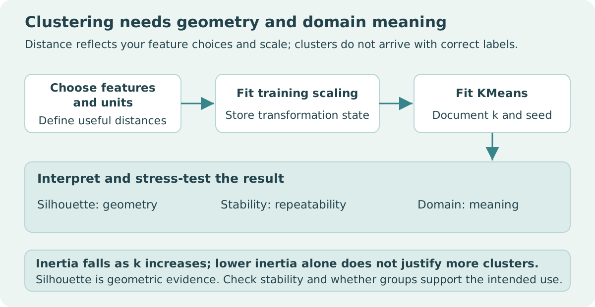
A clustering algorithm returns two labels, and a report immediately calls them two kinds of customers. That conclusion skips the decisions that created the labels: which features were included, their units, the distance metric, the number of clusters, and the fitted solution. An unsupervised algorithm can produce a partition without establishing that the partition describes meaningful categories in the world.
K-means is useful for exploring a chosen Euclidean representation. Silhouette can help inspect separation in that representation. This guide shows how scaling changes the result on a small fixture, explains why inertia alone cannot choose the number of clusters, and separates geometric evidence from stability and domain usefulness.
1. Feature choices define distance
K-means minimizes the sum of squared distances from points to their assigned centers. A feature with large numerical variation can contribute more to those distances than a feature with smaller variation. Changing units can therefore change the fitted partition even when the underlying observations describe the same entities.
Standardization subtracts a fitted mean and scales by a fitted standard deviation for nonconstant features. It gives those features a comparable variance scale, but that is a modeling choice, not a universal correction. If one feature's units already encode the desired relative importance, standardizing may remove a meaningful weighting. If a feature contains extreme outliers, its fitted scale can also be distorted.
Start with the intended similarity question. Are two records close because their absolute values match, their relative profiles match, or particular attributes match? Euclidean distance on arbitrary encoded columns does not answer every version of that question. Category codes, identifiers, and post-outcome fields need particular scrutiny before inclusion.
2. Observe the effect of scaling on the same points
import numpy as np
from sklearn.cluster import KMeans
from sklearn.metrics import silhouette_score
from sklearn.preprocessing import StandardScaler

X = np.array([[0, 0], [0, 40], [1, 80],
              [10, 20], [10, 60], [11, 100]], dtype=float)
scaled = StandardScaler().fit_transform(X)
raw_model = KMeans(n_clusters=2, n_init=20, random_state=7).fit(X)
scaled_model = KMeans(n_clusters=2, n_init=20, random_state=7).fit(scaled)

def partition(labels):
    return sorted(tuple(np.flatnonzero(labels == label))
                  for label in np.unique(labels))

assert partition(raw_model.labels_) == [(0, 1, 3), (2, 4, 5)]
assert partition(scaled_model.labels_) == [(0, 1, 2), (3, 4, 5)]
raw_silhouette = silhouette_score(X, raw_model.labels_)
scaled_silhouette = silhouette_score(scaled, scaled_model.labels_)
assert np.isclose(raw_model.inertia_, 1727.333333, atol=1e-6)
assert np.isclose(scaled_model.inertia_, 5.538578, atol=1e-6)
assert np.isclose(raw_silhouette, 0.495650, atol=1e-6)
assert np.isclose(scaled_silhouette, 0.348635, atol=1e-6)
print("Raw:", partition(raw_model.labels_), raw_silhouette)
print("Scaled:", partition(scaled_model.labels_), scaled_silhouette)
The raw solution primarily separates the larger second-coordinate variation, while the standardized solution separates the two ranges of the first coordinate. The code reports partitions as row-index sets because numeric cluster labels are arbitrary. Label zero in one run does not necessarily identify the same group as label zero in another.
| Representation | Row-index partition | Inertia, rounded | Mean silhouette, rounded |
|---|---|---|---|
| Raw coordinates | {0, 1, 3} and {2, 4, 5} | 1727.333 | 0.496 |
| Standardized coordinates | {0, 1, 2} and {3, 4, 5} | 5.539 | 0.349 |
The two inertia values are measured in different spaces and are not directly comparable as evidence that one preprocessing choice is better. The silhouette values also describe different distance geometries. The larger raw-space score does not establish that raw units match the intended similarity question. The example demonstrates sensitivity, not a winner.
3. Understand what silhouette summarizes
For each sample, silhouette compares its mean distance to other points in its own cluster with its mean distance to the nearest other cluster. The normalized difference is (b - a) / max(a, b). Values near one indicate separation in the chosen distance space; values near zero indicate overlap; negative values suggest a point is closer on average to another cluster.
The mean can hide difficult boundary points or a poorly separated small cluster. Inspect per-sample values and cluster sizes as well as the overall average. Scikit-learn's silhouette calculation requires at least two labels and fewer labels than samples. Asking for one cluster or assigning every observation its own label does not provide a valid silhouette comparison.
import numpy as np
from sklearn.cluster import KMeans
from sklearn.metrics import silhouette_samples, silhouette_score
from sklearn.preprocessing import StandardScaler

X = np.array([[0, 0], [0, 40], [1, 80],
              [10, 20], [10, 60], [11, 100]], dtype=float)
Z = StandardScaler().fit_transform(X)
model = KMeans(n_clusters=2, n_init=20, random_state=7).fit(Z)
sample_scores = silhouette_samples(Z, model.labels_)
assert len(sample_scores) == len(X)
assert np.isclose(sample_scores.mean(), silhouette_score(Z, model.labels_))
for label in np.unique(model.labels_):
    members = np.flatnonzero(model.labels_ == label)
    print("Rows", members.tolist(), "silhouettes", sample_scores[members])
inertias = [KMeans(n_clusters=k, n_init=20, random_state=7).fit(Z).inertia_
            for k in [1, 2, 3]]
assert inertias[0] >= inertias[1] >= inertias[2]
print("Fixture inertia for k=1,2,3:", inertias)
The decreasing inertia is verified for this fixture. At the global optimization level, adding centers expands the set of possible solutions, so the optimal objective cannot increase. A heuristic run can still reach different local solutions. Do not use an unexplained monotonicity assumption to diagnose every numerical result from independently initialized fits.
4. Initialization and repeatability are part of the method
K-means can converge to local solutions, so initialization matters. Set random_state and n_init explicitly when a tutorial or report promises reproducibility. In scikit-learn 1.8, the "auto" setting uses different run counts depending on the initialization method. Writing the intended count avoids hiding that choice behind a changing default.
A fixed seed makes an experiment repeatable under its environment; it does not demonstrate that the partition is stable. Try multiple seeds and appropriate resampled datasets, then compare partitions with a label-invariant measure or matched groups. Report whether important assignments and cluster profiles persist.
Fit any learned scaling inside the relevant training boundary when clusters will be assigned to later unseen data. A purely descriptive analysis of one completed dataset can fit scaling on that dataset, but should be described as such. Transform new rows with the retained scaler instead of refitting it independently and making old centers incompatible with new coordinates.
5. Choosing the number of clusters needs more than one curve
Inertia usually falls as more centers are allowed, so its absolute decrease does not automatically justify additional clusters. An elbow can be a useful visual clue but may be ambiguous. Silhouette examines a different geometric property and also reflects the chosen metric and representation.
Compare several plausible cluster counts alongside size balance, per-cluster profiles, stability, and the intended use. A tiny cluster may reveal a meaningful rare pattern, a data-quality error, or an outlier forced into its own group. Inspect the records before naming it. Do not choose a count solely because one rounded score is slightly larger in a small sample.
K-means and silhouette tend to suit compact, separated geometry better than every possible cluster shape. Curved structures, uneven density, and extensive noise can call for different methods and validation choices. Trying another algorithm still requires an explicit similarity definition and interpretation of its output.
6. Give cluster names only after checking their meaning
Describe observed feature profiles first, with units and counts. Then determine whether proposed names accurately summarize them and whether the groups support the intended decision. Avoid turning arbitrary cluster numbers into ordered rankings or implying that a higher-numbered cluster is inherently better.
For practice, multiply the first coordinate by one hundred and rerun raw-space clustering. Explain why the result can change, then compare it with standardized-space behavior. Finally, remove one point and inspect partition stability. A defensible clustering report identifies feature choices, geometry, initialization, cluster-count selection, stability, and domain evidence; a single attractive silhouette score establishes much less.
Sources and scope
- scikit-learn 1.8: KMeans and initialization.
- scikit-learn 1.8: silhouette_score.
- scikit-learn 1.8: clustering guide.
- scikit-learn 1.8: preprocessing and scaling.
All numerical values come from the displayed six-point fixture. They are not evidence of a natural population structure or a benchmark of clustering algorithms.