Learning Curves: Diagnose Data and Model Limits Without Promising Future Gains
Generate tested train-size curves, read score direction correctly, and distinguish diagnostic patterns from justified predictions about more data.
Reviewed October 9, 2026. Examples use Python 3.12, NumPy 2.3.5, and scikit-learn 1.8.0. Generated observations are synthetic.
A model performs poorly on validation data, and the first proposed solution is to collect more examples. That may be sensible, but a single score does not reveal whether more examples address the limitation. The representation might omit the useful signal, the model might be too constrained, or validation might describe a different population. Learning curves provide a structured diagnostic by showing training and held-out scores at several training sizes.
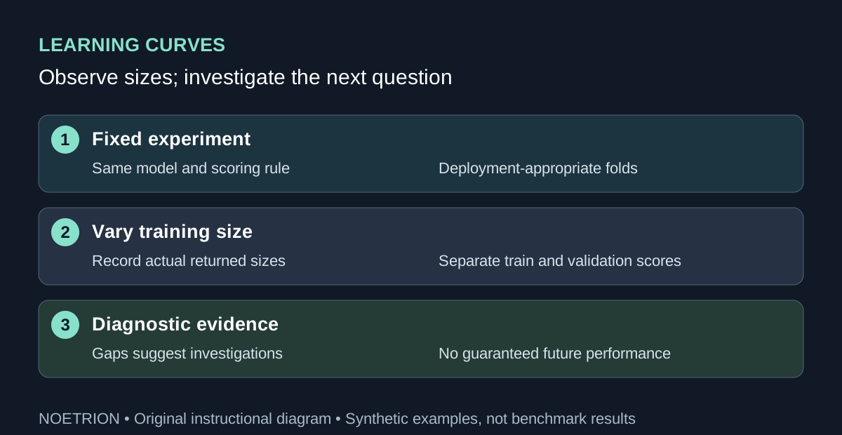
The curve is evidence about the evaluated sizes under a specified sampling and fitting procedure. It is not a guarantee that doubling the dataset will produce a particular gain. This guide builds small reproducible curves, explains their axes and uncertainty, and shows how to connect an observed pattern to a next experiment rather than an unsupported forecast.
1. Specify exactly what changes with size
A learning curve varies the number of training observations while holding a model configuration and scoring rule fixed. A validation curve instead varies a model parameter. Mixing these questions makes the plot hard to interpret: if both training size and regularization change at every point, a rising validation score cannot be attributed to additional data alone.
The learning_curve API returns the actual training sizes and separate score arrays across splits. Fractions in train_sizes refer to available training-fold capacity, not necessarily the full input row count. Always display the returned sizes rather than guessing the horizontal coordinates from the requested fractions.
Write down the prediction unit before generating the curve. Ten thousand rows from ten devices provide a different form of evidence from ten thousand independently sampled devices. If deployment involves unseen entities or future periods, the split and size definition should reflect that condition. A shuffled row curve can be a poor diagnostic for a grouped or chronological deployment question.
2. Generate a curve with an explicit score direction
import numpy as np
from sklearn.datasets import make_regression
from sklearn.linear_model import Ridge
from sklearn.model_selection import KFold, learning_curve
from sklearn.pipeline import make_pipeline
from sklearn.preprocessing import StandardScaler

X, y = make_regression(n_samples=120, n_features=5,
                       noise=10, random_state=4)
estimator = make_pipeline(StandardScaler(), Ridge(alpha=1.0))
cv = KFold(n_splits=3, shuffle=True, random_state=7)
sizes, train, validation = learning_curve(
    estimator, X, y, train_sizes=[0.25, 0.5, 1.0], cv=cv,
    scoring="neg_mean_absolute_error", shuffle=True,
    random_state=11, error_score="raise", n_jobs=1)
assert sizes.tolist() == [20, 40, 80]
assert train.shape == validation.shape == (3, 3)
assert np.isfinite(train).all() and np.isfinite(validation).all()
assert (train <= 0).all() and (validation <= 0).all()
train_mae, validation_mae = -train.mean(axis=1), -validation.mean(axis=1)
for size, tr, va in zip(sizes, train_mae, validation_mae):
    print(int(size), round(float(tr), 3), round(float(va), 3))
Scikit-learn scorers follow a higher-is-better convention, so the negative MAE scorer returns nonpositive values. Negating them produces errors for which lower is better. A plot must label that conversion clearly. Reading an increasing negative score as an increasing error would reverse the conclusion.
The program asserts shape, actual sizes, finiteness, and score direction. It deliberately does not assert that every score improves monotonically with size. Finite samples, subset composition, regularization, and fitting behavior can produce local fluctuations. The printed values belong to this generated regression problem; they are not benchmark measurements for a production dataset.
3. Compare an intentionally limited model with a flexible one
The next fixture creates a quadratic relationship. A linear representation lacks the squared term, while a polynomial representation supplies it. This is a controlled mechanism demonstration: we know the generating relationship because we wrote it. Real data seldom comes with that privilege, so an analogous diagnosis requires additional checks.
import numpy as np
from sklearn.linear_model import LinearRegression
from sklearn.model_selection import KFold, learning_curve
from sklearn.pipeline import make_pipeline
from sklearn.preprocessing import PolynomialFeatures

rng = np.random.default_rng(8)
X = rng.uniform(-2, 2, size=(90, 1))
y = X[:, 0] ** 2 + rng.normal(0, 0.03, size=90)
cv = KFold(n_splits=3, shuffle=True, random_state=2)
linear = LinearRegression()
quadratic = make_pipeline(PolynomialFeatures(2, include_bias=False),
                          LinearRegression())
results = []
for model in (linear, quadratic):
    sizes, train, valid = learning_curve(
        model, X, y, train_sizes=[0.5, 1.0], cv=cv,
        scoring="neg_mean_squared_error", shuffle=True,
        random_state=3, error_score="raise")
    assert sizes.tolist() == [30, 60]
    assert np.isfinite(valid).all()
    results.append(-valid.mean(axis=1))
assert results[1][-1] < results[0][-1]
print("Final-size synthetic MSE:", results[0][-1], results[1][-1])
The last assertion is a fixture-specific result verified by the program. It supports the narrow conclusion that adding the known quadratic feature improves validation error here. It does not prove that polynomial features should be used on every dataset or that collecting more data is unnecessary for this type of problem.
Notice that the two model curves are separate experiments under the same folds and scoring rule. This preserves a readable comparison. If a large search over model families is performed, the selected winner also needs evaluation accounting for that search. Repeatedly selecting the best-looking development curve can overfit the development process itself.
4. Read patterns as hypotheses
The validation and learning curve guide explains their diagnostic purpose. In practice, translate a pattern into a testable next action rather than assigning a permanent label to the dataset. There may be several causes for the same visible shape.
| Observed pattern | Possible explanation | Useful next investigation |
|---|---|---|
| Low training error, much higher validation error | Excess flexibility or mismatch between samples | Simpler model, leakage audit, split review |
| High errors with a small gap | Missing signal or constrained representation | Feature investigation and suitable alternative model |
| Validation error falls over observed sizes | Additional examples may help under this sampling process | A bounded collection experiment with later evaluation |
| Large variation across splits | Unstable subsets or uneven populations | Slice counts, entity structure, repeated diagnostics |
| Sudden break at one size | Composition change or fitting failure | Inspect included rows and failure logs |
A small gap can also occur because training and validation are both contaminated, or because the score is insensitive to an important failure. A large gap can reflect distribution shift rather than ordinary model variance. The table lists plausible explanations, not an automatic classifier for model problems.
5. Treat uncertainty and sampling honestly
Scores from cross-validation folds are not generally independent repeated samples of an untouched deployment population. Their training sets overlap. A standard deviation across folds is a useful descriptive measure, but it should not casually be labeled a formal confidence interval for production performance. State what the displayed band represents and how it was calculated.
Subset order also matters. The API can shuffle training data before taking prefixes, independently of how the outer splitter forms folds. With ordered input and no prefix shuffling, the smallest training subsets may overrepresent a class, period, or source. Some small classification subsets can contain only one class and fail to fit. Use explicit failures during development rather than silently presenting missing scores as evidence of performance.
The cross-validation guide supports choosing a splitter appropriate to the data structure. For time-dependent data, preserve availability and chronology. For repeated entities, ensure the evaluated boundary matches the deployment boundary. Also check whether changing size changes the number of entities, elapsed history, or only records per entity; those are different experiments.
6. Turn the diagnosis into a decision
A collection plan should specify which examples will be added and why they resemble the intended prediction setting. More near-duplicate rows may increase size without improving coverage. Targeting poorly represented cases can be useful, but the evaluation population and labeling process must remain explicit so that the new result answers the same product question.
Keep a final test set separate while using development curves to select features, regularization, and collection strategy. Fit learned preprocessing inside the estimator pipeline, so each fold learns only from its training subset. Record score units, split seeds, actual sizes, estimator parameters, and package versions with the resulting arrays.
Finally, compare the operational cost of the proposed next experiment with the uncertainty it resolves. If the largest observed points are still changing, a modest additional sample may test whether the trend persists. If both errors remain high, inspecting missing signal may be more informative. Learning curves earn their value by narrowing the next question, rather than promising a future accuracy number unsupported by observed data.
Sources and scope
The three official scikit-learn 1.8 references support the curve APIs and validation framework. The generated fixtures and diagnostic table are original instructional material. Their outputs establish local behavior under explicit seeds and splits, not a universal data-size law or a forecast of production improvement.