Permutation Importance: Explain Model Reliance Without Claiming Causation
Measure score decreases under feature perturbation, inspect correlated substitutes, and distinguish repeat variability from population uncertainty.
Reviewed October 8, 2026. Examples target scikit-learn 1.8.0 and use deterministic synthetic data.
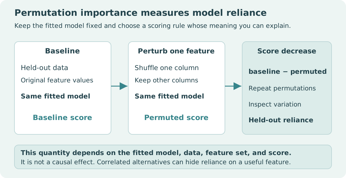
A feature-importance chart often looks like a ranked explanation of reality. Permutation importance supports a narrower statement: how much a particular fitted model's score changes when a particular feature is shuffled in a particular evaluation dataset. Its result depends on the model, the feature set, the scoring rule, and the data on which it is measured.
That narrower interpretation is useful. It can reveal reliance on a feature, compare training and held-out behavior, and help inspect a prediction pipeline. It cannot by itself establish a causal effect, prove that a low-ranked feature contains no useful information, or decide which fields should be removed without further evaluation.
1. Define the baseline and the perturbation
Start with a fitted estimator and an evaluation dataset. Compute a baseline score using the unchanged inputs. Shuffle one feature across rows while keeping the estimator fixed, compute the score again, and subtract the perturbed score from the baseline. Repeat shuffles to observe how the result varies under that perturbation process.
The direction of the scoring rule matters. Scikit-learn's scorer convention makes larger scores better, including negative versions of error losses. Under that convention, a positive baseline-minus-perturbed difference means the shuffle worsened the score. If manually using a positive error loss, define the difference in the opposite direction or explain it carefully.
First verify that the model predicts meaningfully on the evaluation data. A poor model may ignore a genuinely informative feature because it failed to learn its relationship. A low permutation importance for that model is not evidence that the underlying variable has no predictive information.
2. Inspect a controlled correlated-feature example
The fixture below uses two identical predictors. Training and evaluation rows are separate, although the relationship is deliberately trivial and does not represent a realistic prediction task. A fixed reverse-row permutation makes the arithmetic transparent.
import numpy as np
from sklearn.linear_model import LinearRegression
from sklearn.metrics import r2_score

train_x = np.arange(8.0)
test_x = np.arange(8.0, 12.0)
X_train = np.column_stack([train_x, train_x])
X_test = np.column_stack([test_x, test_x])
model = LinearRegression().fit(X_train, train_x)
assert np.allclose(model.coef_, [0.5, 0.5])
baseline = r2_score(test_x, model.predict(X_test))
first_only = X_test.copy()
first_only[:, 0] = first_only[::-1, 0].copy()
both = X_test[::-1].copy()
first_score = r2_score(test_x, model.predict(first_only))
both_score = r2_score(test_x, model.predict(both))
assert np.isclose(baseline, 1.0)
assert np.isclose(first_score, 0.0)
assert np.isclose(both_score, -3.0)
print("Score decreases:", baseline - first_score, baseline - both_score)
When only the first feature is reversed, the two half-weighted inputs average to 9.5 for every test row. That is the evaluation target's mean, so the R² score becomes zero. Reversing both features together reverses the predictions and gives a score of negative three. The corresponding score decreases are one and four.
| Fixed perturbation | R² on the four evaluation rows | Baseline score decrease |
|---|---|---|
| None | 1 | 0 |
| Reverse first column only | 0 | 1 |
| Reverse both identical columns together | −3 | 4 |
The joint perturbation is a separate group-reliance experiment, not the standard one-column API result. The fixture demonstrates interaction between correlated inputs and perturbation choice. It does not establish a universal numerical relationship between individual and group importance.
3. Use repeated random shuffles for the API quantity
import numpy as np
from sklearn.inspection import permutation_importance
from sklearn.linear_model import LinearRegression

train_x = np.arange(8.0)
test_x = np.arange(8.0, 12.0)
X_train = np.column_stack([train_x, train_x])
X_test = np.column_stack([test_x, test_x])
model = LinearRegression().fit(X_train, train_x)
result = permutation_importance(model, X_test, test_x, scoring="r2",
                                n_repeats=10, random_state=7)
assert result.importances.shape == (2, 10)
assert np.isfinite(result.importances).all()
assert np.allclose(result.importances_mean, [0.5, 0.5])
assert (result.importances_std > 0).all()
print("Means:", result.importances_mean)
print("Shuffle standard deviations:", result.importances_std)
The mean score decreases are 0.5 for each feature under this exact ten-repeat fixture and seed. They differ from the fixed reverse permutation because the API averages different shuffles. Those decimals are reproducibility checks, not population feature-importance estimates from a substantive dataset.
The reported standard deviation describes variation across shuffles of these same rows. It is not a confidence interval for a population quantity and does not incorporate uncertainty from training-sample selection, model fitting, or dataset shift. More repeats stabilize the perturbation average without creating more independent evaluation subjects.
4. Correlated alternatives change the interpretation
If one feature has a close substitute, the model may retain much of its predictive ability when either is shuffled separately. Individual importances can then look small even when the information shared by the pair matters. The effect depends on how the fitted estimator uses those features; correlation does not force one universal outcome.
Standard marginal shuffling can also generate combinations that are unusual or impossible under the original joint distribution. For example, a derived total may cease to agree with its component columns. The score change then reflects model behavior on those perturbed combinations, which may differ from plausible changes in the real system.
Possible investigations include grouping related fields for a joint perturbation, clustering correlated features and choosing representatives, or retraining after removing a feature group. These answer different questions. Retraining measures what another model can learn without the fields; keeping the model fixed measures the existing model's reliance. Label the distinction rather than comparing both results as if they were interchangeable.
5. Preserve the evaluation boundary and feature meaning
Use held-out data when the question concerns reliance that generalizes beyond training. A training importance can reveal memorization, but should not be advertised as held-out evidence. Group and time boundaries must still match the deployment task, as in any other evaluation.
For a pipeline receiving raw tabular columns, perturbing the raw feature and passing it through the fitted preprocessing can preserve a meaningful unit of inspection. Permuting individual one-hot columns independently can create an invalid category representation. Decide whether the explanation concerns original fields, transformed columns, or groups of derived features.
Time-dependent and grouped data introduce another assumption: freely shuffling values across all rows may break structure that matters. A restricted perturbation may be more appropriate for a specific question, but its design and interpretation need justification. Do not present a convenient unrestricted shuffle as a valid causal experiment simply because it produces a chart.
6. Report enough detail to reproduce the claim
A feature-removal decision should also consider collection cost, availability, redundancy, and robustness. A highly relied-on field may be unusable because it arrives after the decision time; a low individual importance may belong to a valuable redundant measurement that protects against another sensor's failure. Reevaluate the actual candidate pipeline after changing its inputs. The importance chart is evidence about an existing model, while the operational decision concerns a proposed workflow and its supported conditions.
Record the model version, evaluation rows, baseline performance, feature set, scorer, repeat count, seed, and perturbation method. Include the sign convention and relevant correlations. Negative importance can arise from variability or a perturbation improving a model's score; it deserves investigation rather than automatic deletion.
For practice, fit a model using only one of the duplicated columns and compare its importance with the two-column model. Then compare held-out baseline performance after removing a field and retraining. Explain why that result concerns a different fitted estimator. A defensible feature-importance report describes observable reliance and its limits rather than naming the bars “causes.”
Sources and scope
- scikit-learn 1.8: permutation feature importance.
- scikit-learn 1.8: correlated-feature example.
- scikit-learn 1.8: permutation_importance API.
- scikit-learn 1.8: scoring and metrics.
The original four-row evaluation fixture demonstrates mechanics only. No real-world importance, causal effect, or model-performance benchmark is claimed.