Probability Calibration: Check Reliability Without Confusing It with Ranking
Understand what calibrated probabilities mean, inspect bin counts, calculate binary Brier loss, and avoid treating a lower loss as isolated proof of better calibration.
Reviewed October 6, 2026. Examples use Python 3.12.14 and scikit-learn 1.8.0. All outcomes are constructed; the small fixtures illustrate definitions rather than establish a real model's calibration.
A classifier labels a case with probability 0.8. Does that mean it is correct 80% of the time? The question is incomplete. Calibration concerns groups of predictions and their observed outcome frequencies under an evaluation population, not a guarantee about one individual case.
A model can rank positive cases above negative cases while producing badly interpreted probabilities. Another can match overall prevalence with a constant probability while offering no useful separation among individual cases. Reliability and discrimination are related aspects of evaluation, but neither substitutes for the other.
Practical rule: inspect probability reliability with sample counts and appropriate held-out data, evaluate ranking separately, and use Brier loss as a overall probabilistic score rather than a pure calibration measure. Keep the calibration procedure outside the final test set.
What a reliability diagram compares
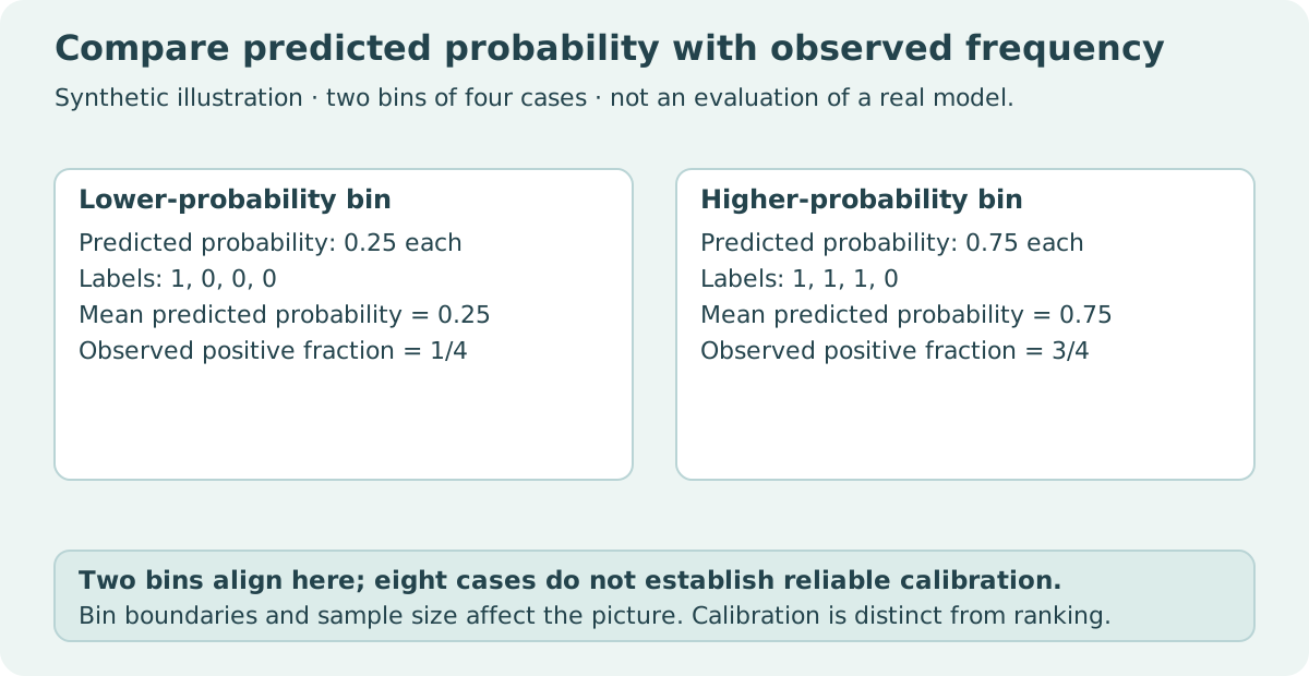
A reliability diagram groups predictions into bins, then compares the average predicted probability in each bin with its empirical positive fraction. If four cases all receive probability 0.25 and one is positive, that bin aligns exactly in the observed fixture.
The bin is still only four observations. Its apparent agreement can be fragile. A useful diagram displays bin counts or a companion histogram so readers see where the estimated frequencies have substantial evidence and where they do not.
from sklearn.calibration import calibration_curve

labels = [1, 0, 0, 0, 1, 1, 1, 0]
probabilities = [0.25] * 4 + [0.75] * 4
observed, predicted = calibration_curve(labels, probabilities, n_bins=2, strategy="uniform")
assert observed.tolist() == [0.25, 0.75]
assert predicted.tolist() == [0.25, 0.75]
counts = [sum(p < 0.5 for p in probabilities), sum(p >= 0.5 for p in probabilities)]
assert counts == [4, 4]
print({"predicted": predicted.tolist(), "observed": observed.tolist(), "counts": counts})
| Bin | Cases | Mean predicted probability | Observed positive fraction |
|---|---|---|---|
| Lower | 4 | 0.25 | 1/4 = 0.25 |
| Higher | 4 | 0.75 | 3/4 = 0.75 |
The threshold 0.5 used to count these constructed bins is not a recommended classification threshold. Binning for reliability and choosing a decision threshold are separate operations. Real bin boundaries must be recorded alongside the plot.
Bin design changes what you can see
Uniform bins use intervals of equal probability width. Quantile bins aim to group observations by their distribution of predicted probabilities. Either can reveal a different picture, especially when most predictions occupy a narrow score range.
More bins provide a finer view but fewer observations in each bin. Fewer bins can hide local failures behind an average. Empty bins do not carry an empirical outcome estimate; do not plot them as if a zero positive rate had been observed.
The scikit-learn calibration guide describes reliability diagrams and calibration procedures. Treat the curve as an estimate under the supplied sample, with uncertainty and grouping choices. A small diagonal-looking plot is not proof of calibration across future populations, subgroups, or time periods.
If subgroup performance matters to the application, evaluate those populations separately with adequate evidence. Aggregate agreement can coexist with different subgroup reliability. This article does not infer subgroup behavior from its eight synthetic cases.
Binary Brier loss is a squared probability error
For binary outcomes, calculate the average of (probability minus outcome) squared. Lower values reward probabilities close to the observed labels. The score evaluates probabilistic predictions, but it combines more than calibration alone.
from sklearn.metrics import brier_score_loss

def binary_brier(labels, probabilities):
    if len(labels) != len(probabilities) or not labels:
        raise ValueError("equal nonempty sequences required")
    if any(type(label) is not int or label not in (0, 1) for label in labels):
        raise ValueError("labels must be binary integers")
    if any(not 0 <= probability <= 1 for probability in probabilities):
        raise ValueError("probabilities must be between 0 and 1")
    return sum((probability - label) ** 2 for label, probability
               in zip(labels, probabilities)) / len(labels)

labels = [0, 0, 1, 1]
constant = [0.5, 0.5, 0.5, 0.5]
sharper = [0.1, 0.1, 0.9, 0.9]
assert binary_brier(labels, constant) == 0.25
assert abs(binary_brier(labels, sharper) - 0.01) < 1e-12
assert abs(brier_score_loss(labels, sharper) - 0.01) < 1e-12
print("Constant:", binary_brier(labels, constant))
print("Sharper:", binary_brier(labels, sharper))
The helper's accepted probability inputs are ordinary numeric values compatible with its operations; it is not a general parser for arbitrary documents. Under that stated input domain, a nonfinite value cannot satisfy the range check. A production boundary should also state its numeric type and Boolean policy explicitly.
| Predictions on four constructed cases | Brier loss | Empirical reliability view |
|---|---|---|
| Constant 0.5 | 0.25 | One bin predicts 0.5 and observes 0.5 |
| 0.1 for negatives, 0.9 for positives | 0.01 | Bins observe 0 and 1 rather than 0.1 and 0.9 |
The sharper predictions have much lower Brier loss because they separate the outcomes well. The constant predictor exactly matches the fixture's overall positive fraction but has no individual discrimination. Lower Brier therefore does not isolate “better calibration.” The calibration guide discusses reliability, resolution, and uncertainty as components of its interpretation.
Both statements concern these four records only. Calling either system population-calibrated from this sample would overstate the evidence. The fixture is a counterexample to an inference about a metric, not a validated real model comparison.
Calibration requires independent predictions
A calibrator learns a mapping from model scores to probabilities. If you fit that mapping using predictions from the same cases the base model was trained to fit, optimistic training behavior can contaminate the mapping. Use an appropriate held-out or cross-validated prediction design.
Keep a separate final evaluation population. Using the test set to choose the calibration method, tune its parameters, and report its final result turns the test set into development data. Temporal and grouped dependencies require additional splitting care; a nominally separate random subset may still leak relevant information.
| Stage | Permitted role | Boundary to maintain |
|---|---|---|
| Base-model training | Fit model parameters | Do not use final test outcomes |
| Calibration | Fit probability mapping from independent scores | Do not reuse optimistic fitted-case predictions blindly |
| Method selection | Compare supported alternatives | Keep final evaluation independent |
| Final evaluation | Estimate reliability, ranking, and decision results | Do not tune the final mapping here |
The exact procedure depends on the model and available data. This article teaches the independence requirement without prescribing a universal fold count or minimum sample size.
A mapping can affect ties and decision behavior
A strictly increasing transformation preserves ordering, although it changes numeric threshold meanings. A calibration method that introduces ties can affect ranking metrics. Isotonic calibration, for example, can produce flat portions, so do not promise that every calibration procedure leaves AUC identical.
After calibration, re-evaluate both the probability interpretation and the selected decision policy. A fixed threshold such as 0.5 can select a different population after the mapping, even when much of the ranking remains similar. The decision should follow the application's costs, capacity, and validated probability use.
Calibration can also drift when the population or data collection process changes. A mapping fitted under one prevalence and score distribution does not automatically establish reliability under every future distribution. Monitor the actual evaluation population when outcomes become available.
Report more than one attractive number
A useful report includes the evaluation period, sample size, positive count, split design, reliability binning strategy, bin counts, Brier loss definition, and a ranking measure. For decisions, include threshold-specific counts and rates. State whether calibration was fitted before or after the base model and which data each stage used.
For reproducibility across library versions, the direct binary formula above avoids relying on newly introduced multiclass scaling arguments. If your task is multiclass, document the exact Brier definition and scaling rather than comparing unlike values under one name.
The aim is to make “probability 0.8” a checkable population-level interpretation, while keeping ranking quality and decision usefulness visible as separate evidence.
Sources and reproducibility
Primary references: scikit-learn 1.8 calibration guide, calibration_curve, and Brier score loss. Both examples run independently. They illustrate definitions and counterexamples; no calibrator was fitted or real classifier benchmarked.