Regression Metrics: Read MAE, RMSE, and R² as Different Error Contracts
Calculate three regression metrics by hand, compare mean and median references, and explain units, negative R-squared, weighting, and constant-target edge cases.
Reviewed October 8, 2026. Examples target scikit-learn 1.8.0 and use synthetic target values.
A regression model receives three numbers in an evaluation report: MAE, RMSE, and R². They are not three interchangeable descriptions of “accuracy.” They summarize errors differently and answer different questions. A model can have a modest mean absolute error while a small number of large mistakes substantially raises its root mean squared error.
This article works through a four-row fixture with a known answer, explains the units and reference used by each metric, and shows why negative R² is possible. It also separates the mathematical reference inside R² from a deployable baseline fitted using training data. No model-performance claim is inferred from the synthetic numbers.
1. Start with paired predictions and observations
Every metric requires the correct prediction to be paired with the correct observed target. An index mismatch can produce a plausible score for unrelated rows. Retain record IDs and verify row order or join keys before calculation. Also state which observations are included, how missing outcomes are handled, and whether repeated entities receive equal weight.
MAE is the average absolute residual. RMSE is the square root of the average squared residual. Both have the target's units, but RMSE penalizes large residuals more strongly through squaring. R² compares the model's squared-error sum with the squared deviations around the evaluation target's mean, yielding a dimensionless relative score.
These definitions do not select a business loss function. If underprediction and overprediction have different costs, or some errors trigger thresholds, the relevant loss may be asymmetric or task-specific. Common metrics are useful summaries, but the decision rule should explain why their treatment of errors matches the use case.
2. Reproduce the arithmetic
import numpy as np
from sklearn.metrics import mean_absolute_error, root_mean_squared_error, r2_score

y = np.array([0.0, 0.0, 0.0, 10.0])
prediction = np.zeros(4)
residual = y - prediction
mae = mean_absolute_error(y, prediction)
rmse = root_mean_squared_error(y, prediction)
reference_sse = np.sum((y - y.mean()) ** 2)
model_sse = np.sum(residual ** 2)
r2 = r2_score(y, prediction)
assert mae == 2.5
assert rmse == 5.0
assert reference_sse == 75.0 and model_sse == 100.0
assert np.isclose(r2, -1 / 3)
print({"MAE": mae, "RMSE": rmse, "R2": r2})
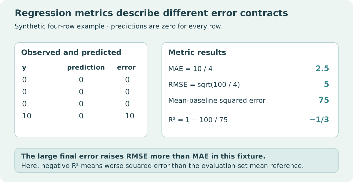
The absolute errors sum to ten, so MAE is ten divided by four. Squared errors sum to one hundred, so RMSE is the square root of one hundred divided by four. The evaluation mean is 2.5, and the squared deviations around it sum to seventy-five. R² is therefore 1 - 100 / 75, or negative one-third.
| Metric | Calculation in this fixture | Result | Interpretation |
|---|---|---|---|
| MAE | (0 + 0 + 0 + 10) / 4 | 2.5 | Average absolute error in target units |
| RMSE | sqrt((0 + 0 + 0 + 100) / 4) | 5 | Squared-error emphasis, returned to target units |
| R² | 1 − 100 / 75 | −1/3 | Worse squared error than the evaluation-mean reference |
For a single-output dataset with the same nonnegative weighting scheme, RMSE is at least MAE. That mathematical relationship does not mean a larger RMSE identifies a worse model than a different model's MAE. Compare like with like on the same observations and weights.
3. Mean and median references optimize different losses
For this completed fixture, predicting its mean minimizes squared error among constant predictions. Predicting its median minimizes absolute error among constants. The median is zero, so the original all-zero predictions give a lower MAE than constant 2.5, even though their squared error is worse.
import numpy as np
from sklearn.metrics import mean_absolute_error, root_mean_squared_error, r2_score

y = np.array([0.0, 0.0, 0.0, 10.0])
median_prediction = np.full(4, np.median(y))
mean_prediction = np.full(4, y.mean())
assert mean_absolute_error(y, median_prediction) == 2.5
assert mean_absolute_error(y, mean_prediction) == 3.75
assert root_mean_squared_error(y, mean_prediction) < root_mean_squared_error(y, median_prediction)
assert r2_score(y, mean_prediction) == 0.0
scale = 100.0
assert np.isclose(mean_absolute_error(y * scale, median_prediction * scale), 250.0)
assert np.isclose(root_mean_squared_error(y * scale, median_prediction * scale), 500.0)
assert np.isclose(r2_score(y * scale, median_prediction * scale), -1 / 3)
print("Loss choice changes the preferred constant; a unit change rescales errors.")
These constants use the evaluation outcomes to illustrate metric definitions. They are not deployable predictions for outcomes not yet observed. In a real evaluation, fit a baseline's mean or median using training outcomes and apply that fixed value to held-out rows. Report its actual held-out errors separately from the mathematical reference in R².
Choosing a model by MAE can select a different model than choosing by RMSE. State which criterion governs selection before examining final evaluation results. Otherwise a report can switch metrics after seeing which one makes a favored model look better.
4. Units and target variation affect comparison
Multiplying both targets and predictions by one hundred multiplies MAE and RMSE by one hundred. R² stays unchanged under that common scaling when its denominator is nonzero. A unit conversion should therefore be visible in the error report, while a dimensionless metric still needs context about the population and target.
R² from two different datasets is not a universal ranking of model usefulness. Its denominator depends on variation in the evaluation target. A narrow-range dataset can produce a poor relative score with small absolute errors; a wide-range dataset can produce a high relative score while errors remain operationally unacceptable. Include error magnitudes and the target distribution rather than relying on one normalized score.
R² is also not generally the square of a correlation between predictions and targets. Predictions with a biased level or wrong scale can correlate strongly with the target and still have a poor R². Inspect residuals and calibration of the regression output rather than substituting correlation for the evaluation metric.
5. Constant targets and weighting require explicit policy
When every evaluation target is the same, the ordinary R² denominator is zero. Scikit-learn defaults to finite replacements for this case: one for perfect predictions and zero for imperfect predictions. Setting force_finite=False exposes nonfinite results instead. A finite replacement is a library convenience, not evidence that a constant-target fold provides the usual relative comparison.
With fewer than two samples, R² is not well-defined. Tiny folds, rare slices, or aggressive filtering can create these cases. Check counts and target variation before interpreting the reported number. Handle them visibly in aggregation rather than silently treating all fold scores as equally informative.
Sample weights change the population being summarized. Equal row weights, equal participant weights, and cost weights answer different questions. Multiple target outputs introduce another aggregation decision: errors in different units should not be averaged casually. Report per-output metrics or justify the normalization and weighting used to combine them.
6. Inspect residuals beyond the averages
An aggregate can hide consistent underprediction for one subgroup, increasing error over time, or a small tail of extreme mistakes. Plot or tabulate residuals against predicted values, relevant groups, and time when appropriate. Preserve the evaluation boundary while choosing those checks, and avoid claiming a stable subgroup result from a handful of observations.
For practice, replace the final prediction of zero with eight and compute all three metrics by hand. Then change one of the first predictions to four and explain how the tradeoff differs under absolute and squared error. A reviewable regression report includes paired data, units, weighting, a training-fitted baseline, several relevant summaries, and clearly stated limitations.
Sources and scope
- scikit-learn 1.8: regression metrics and scoring.
- scikit-learn 1.8: root_mean_squared_error.
- scikit-learn 1.8: r2_score edge cases.
- scikit-learn 1.8: DummyRegressor baselines.
The numerical results are calculated from the displayed original fixture. They do not estimate an error rate for any real application.