ROC and Precision–Recall Curves for Rare Events: Translate Rates into Workload
Understand ranking curves, operational false-positive counts, changing prevalence, and why average precision differs from trapezoidal PR area.
Reviewed October 6, 2026. Examples use Python 3.12.14 and scikit-learn 1.8.0. All scores and labels are constructed demonstrations, not model performance measurements on real events.
A model's ROC curve appears impressive, but its alert queue is dominated by false positives. The contradiction is only apparent: a small false-positive rate applied to a large negative population can create many false alerts. A curve needs its population, threshold, and operational interpretation.
ROC describes true-positive rate against false-positive rate across score thresholds. Precision–recall describes precision against recall. They emphasize different relationships and are both useful when their denominators and summaries are understood.
Practical rule: use curves to compare ranking behavior, then evaluate selected thresholds as counts under the target population. Report prevalence and the exact area metric used. A model's ranking score, probability calibration, and decision policy are separate properties.
Translate a conditional rate into a count
True-positive rate is TP divided by actual positives. False-positive rate is FP divided by actual negatives. Precision is TP divided by predicted positives. A rate conditional on the true class is therefore not the same as the fraction of alerts that are correct.
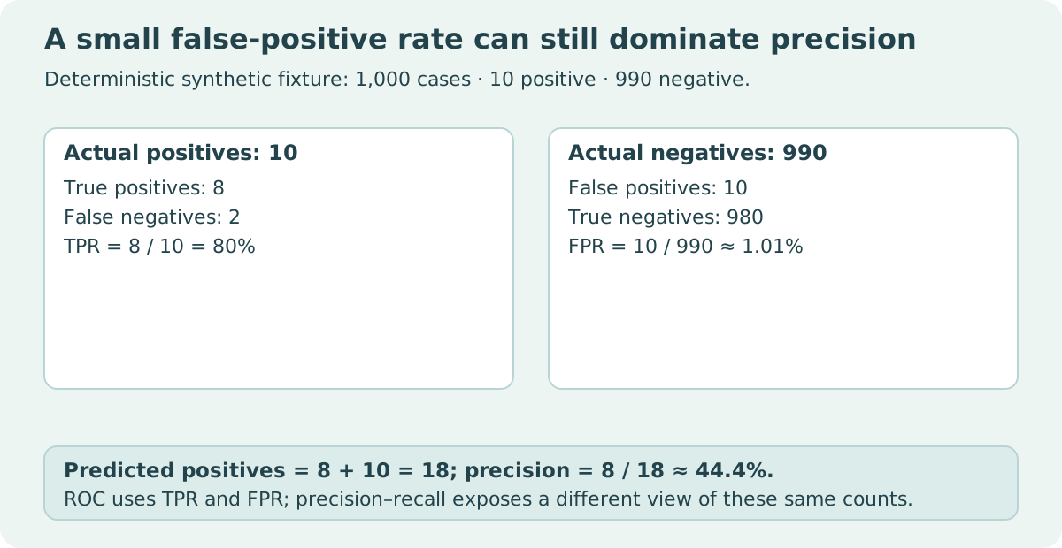
Construct a population of 1,000 cases containing ten positives and 990 negatives. At one threshold, the scores select eight positives and ten negatives. Recall is 80%, FPR is about 1.01%, and precision is about 44.44%. The queue contains eighteen alerts, of which ten are false.
labels = [1] * 10 + [0] * 990
scores = [0.9] * 8 + [0.1] * 2 + [0.8] * 10 + [0.05] * 980
threshold = 0.5
predictions = [score >= threshold for score in scores]
tp = sum(label == 1 and prediction for label, prediction in zip(labels, predictions))
fp = sum(label == 0 and prediction for label, prediction in zip(labels, predictions))
fn = sum(label == 1 and not prediction for label, prediction in zip(labels, predictions))
tn = sum(label == 0 and not prediction for label, prediction in zip(labels, predictions))
assert (tp, fp, fn, tn) == (8, 10, 2, 980)
assert tp / (tp + fn) == 0.8
assert abs(fp / (fp + tn) - 10 / 990) < 1e-12
assert abs(tp / (tp + fp) - 8 / 18) < 1e-12
print({"alerts": tp + fp, "precision": tp / (tp + fp), "recall": tp / (tp + fn)})
| Measure at threshold 0.5 | Calculation | Value |
|---|---|---|
| Recall / TPR | 8 / 10 | 80% |
| FPR | 10 / 990 | About 1.01% |
| Precision | 8 / 18 | About 44.44% |
| Alert workload | 8 + 10 | 18 cases |
The data deliberately contain tied scores. The threshold accepts a complete tied group rather than pretending individual equal-score cases can be ranked separately. A real alert workflow also needs capacity, delay, and error-cost considerations, which this fixture does not estimate.
Prevalence changes the precision relationship
Let prevalence be the fraction of actual positives. If TPR and FPR are held fixed by assumption, precision follows from the expected positive and negative counts. A lower prevalence can reduce precision even though those conditional rates remain the same.
from fractions import Fraction

population = 10000
scenarios = []
for positives in [100, 1000]:
    negatives = population - positives
    tp = Fraction(4, 5) * positives
    fp = Fraction(1, 20) * negatives
    precision = tp / (tp + fp)
    scenarios.append((positives, int(tp), int(fp), float(precision)))
assert scenarios[0][:3] == (100, 80, 495)
assert scenarios[1][:3] == (1000, 800, 450)
assert abs(scenarios[1][3] - 0.64) < 1e-12
print(scenarios)
| Constructed prevalence | Positives | TP at TPR 0.8 | FP at FPR 0.05 | Precision |
|---|---|---|---|---|
| 1% | 100 | 80 | 495 | About 13.91% |
| 10% | 1,000 | 800 | 450 | 64% |
Holding conditional rates fixed is a mathematical scenario, not a claim that a deployed model's rates stay fixed after distribution changes. Changes in input characteristics can alter ranking behavior as well as prevalence. Re-evaluate the actual deployment population rather than mechanically transplanting a validation curve.
A curve evaluates many thresholds, not one decision
The ROC curve reference describes its threshold-dependent coordinates. ROC AUC summarizes ranking across the curve; it does not directly tell you the precision or workload at a selected cutoff.
The precision–recall reference includes an initial point representing every sample predicted positive, whose precision equals prevalence and recall equals one. Its final point at precision one and recall zero has no corresponding threshold. Handle that endpoint carefully when pairing threshold values with displayed coordinates.
A high area can hide poor behavior in the narrow threshold region your workflow uses. If only a small number of cases can be reviewed, inspect the relevant high-score region, the tie policy, and the selected count. Curves describe possibilities; a threshold and capacity policy choose a particular operation.
Average precision is not trapezoidal PR area
Average precision weights precision values by changes in recall. Trapezoidal integration draws straight lines between points. They are different summaries and can differ substantially, especially with coarse or tied scores.
from sklearn.metrics import average_precision_score, precision_recall_curve, auc, roc_auc_score

labels = [0, 0, 0, 1]
scores = [0.1, 0.1, 0.1, 0.1]
precision, recall, thresholds = precision_recall_curve(labels, scores)
ap = average_precision_score(labels, scores)
trapezoidal = auc(recall, precision)
roc_area = roc_auc_score(labels, scores)
assert ap == 0.25
assert trapezoidal == 0.625
assert roc_area == 0.5
assert len(precision) == len(thresholds) + 1
print({"AP": ap, "trapezoidal_PR_area": trapezoidal, "ROC_AUC": roc_area})
| Constant-score fixture | Value | Interpretation |
|---|---|---|
| Average precision | 0.25 | Matches this fixture's positive prevalence |
| Trapezoidal PR area | 0.625 | Different interpolated area definition |
| ROC AUC | 0.5 | No ranking separation from identical scores |
Calling 0.625 “average precision” would be incorrect. The average precision documentation explicitly distinguishes its calculation from trapezoidal area. Name the metric in reports and code rather than using PR AUC as an ambiguous label.
Ranking, calibration, and thresholds need separate evidence
ROC and PR curves consume scores; those scores need not be calibrated probabilities. A monotonic transformation can preserve score ordering while changing the meaning of its numeric values. Choosing 0.5 because a field looks like a probability is not justified unless the probability interpretation has been evaluated.
Use data independent of model training to choose a threshold, and retain a separate final evaluation set. Selecting the most flattering threshold on the final test set turns that set into a tuning resource. For temporal or grouped data, the split must also reflect the deployment's information availability and entity relationships.
Report counts alongside rates. Small numbers of actual positives can make a curve unstable, and resampling or uncertainty analysis requires a design appropriate to how cases were collected. The tiny demonstrations here expose formulas; they do not establish statistical confidence in a real detector.
Ties and incomplete class populations need explicit handling
A score tie is a group of cases with the same threshold status. If a review queue has room for only some of those cases, specify the secondary selection policy. An arbitrary input order can otherwise influence which cases are reviewed while the reported score threshold appears unchanged. Evaluate the complete decision rule, including that tie handling.
A dataset or fold containing only one class cannot establish every ranking comparison. Inspect metric warnings and undefined values rather than replacing them with a convenient zero or copying a score from another fold. Record positive and negative counts for every evaluated population.
Pooling predictions from several fitted models also deserves care: their score scales may differ. A pooled curve can compare scores across models rather than only within one model's ranking. Report fold-specific results and explain any pooling or weighting. Precision-oriented summaries also depend on the evaluated positive population, so compare candidate models on the same held-out cases when attributing a difference to the model.
A useful evaluation report
State the positive event definition, score direction, sample counts, prevalence, split design, and selected threshold. Include its confusion matrix, predicted-positive count, recall, precision, and FPR. If you include an area summary, name AP or trapezoidal area explicitly and document the implementation.
Then connect the chosen threshold to the decision process: how many cases can be handled, what delays matter, and which errors have meaningful costs? Those operational requirements decide where on the curve to work. Neither “ROC is useless for imbalance” nor “PR is always better” replaces that analysis.
Sources and reproducibility
Primary references: ROC curve, precision–recall curve, and average precision. All three examples execute independently. The final example requires scikit-learn; no model was trained or benchmarked.