AI Data Centre Capacity: A Local Power and Scenario Worksheet
Calculate annual electricity, peak connection needs, flexible workload requirements, and tariff exposure with a transparent synthetic facility model.
A global electricity forecast cannot tell you whether a particular data centre has enough power at a particular hour. A site can have a manageable annual energy budget and still exceed its connection capacity during a busy period. Start a local worksheet by separating energy, power, operating conditions, and the computing work that can move in time.
The IEA’s Electricity 2026 report discusses the importance of grids and flexibility as demand expands. This companion uses original synthetic inputs to explain the arithmetic. It is a planning exercise, not a facility design, an electrical operating instruction, or a forecast for a real site.
Write the units beside every input
| Input | Illustrative value | Meaning |
|---|---|---|
| Average IT load | 500 kW | Mean computing-equipment power in the simplified year. |
| Peak IT load | 900 kW | Highest modeled coincident computing load. |
| PUE | 1.40 | Total facility energy divided by IT energy over a matched period. |
| Available firm connection | 1,000 kW | Assumed usable connection capacity for this exercise. |
| Energy price | $0.10/kWh | Flat synthetic tariff excluding other charges. |
A kilowatt is a rate; a kilowatt-hour is energy used over time. Record whether a supplied figure describes IT equipment or the whole facility. Also record the measurement interval. Multiplying an annual-average PUE by an instantaneous peak is only a simplified assumption here; real peak overhead requires a matched operational model.
Calculate annual energy and its limited meaning
With average IT power of 500 kW and a constant modeled PUE of 1.40, average facility power is 500 × 1.40 = 700 kW. For a non-leap year of 8,760 hours, energy is 700 × 8,760 = 6,132,000 kWh, or 6,132 MWh. The corresponding synthetic energy charge is $613,200.
This calculation does not include demand charges, time-of-use prices, taxes, outages, expansion, or equipment variation. It also assumes the average load already accounts for idle periods. If you instead multiply installed maximum load by every hour, label that as a maximum-load scenario rather than measured consumption.
Find the peak capacity gap
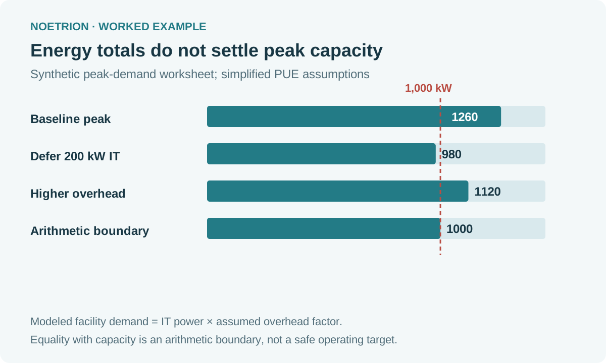
Applying the exercise’s PUE assumption to the 900 kW IT peak gives 1,260 kW of facility demand. Against the 1,000 kW connection, the modeled gap is 260 kW. Reducing annual energy by a few percent elsewhere does not necessarily close that gap. The reduction must occur during the relevant peak.
| Scenario | IT load | Modeled PUE | Facility demand |
|---|---|---|---|
| Baseline peak | 900 kW | 1.40 | 1,260 kW |
| Defer 200 kW of IT work | 700 kW | 1.40 | 980 kW |
| Same deferral, higher overhead | 700 kW | 1.60 | 1,120 kW |
| Higher-overhead case at capacity | 625 kW | 1.60 | 1,000 kW |
At PUE 1.60, keeping modeled facility power within 1,000 kW requires IT load no higher than 625 kW. From the original 900 kW peak, that means deferring 275 kW, not 200 kW. Actual headroom and engineering margins would need additional site-specific analysis; the last row is an arithmetic boundary, not an operating target.
Ask whether the work can really move
List workload deadlines, required hardware, checkpoint behavior, restart cost, and service dependencies. An overnight training job may have scheduling flexibility that an interactive service lacks. Deferring work also moves energy into another period; it does not automatically remove the energy requirement. Check whether the receiving period has sufficient capacity and whether the completion deadline remains achievable.
For each proposed flexibility action, record who owns it, what service it affects, the allowed duration, and how the system returns to normal. Evaluate those constraints with qualified site and service teams before treating a scheduling idea as dependable capacity.
Stress the bill separately from capacity
Keep annual modeled energy at 6,132,000 kWh but change the flat tariff from $0.10 to $0.13. The energy charge becomes $797,160, an increase of $183,960. Neither the computing volume nor the peak load changed. A financial sensitivity and a connection-capacity sensitivity are different parts of the same worksheet.
Complete the worksheet with observed values when available, clearly marking estimates and missing information. It should produce a list of evidence requests: interval load records, matched overhead measurements, connection terms, tariffs, and workload flexibility. For broader sector context, see the electricity behind AI.