Classification Thresholds: Connect Scores to Costs Without Tuning on the Test Set
Derive a conditional expected-cost threshold, test empirical threshold selection, and preserve independent training, tuning, and test boundaries.
Reviewed October 9, 2026. Examples use Python 3.12, NumPy 2.3.5, and scikit-learn 1.8.0. Labels, scores, and cost units are synthetic.
A classifier can rank examples well while making unsuitable yes-or-no decisions. The decision boundary translates a score into an action, and the consequences of that action may not match the default threshold. In a generic routing workflow, missing a case that needs review can have a different operational cost from sending an unnecessary case to review.
Changing a threshold does not retrain the ranking function or make its probabilities calibrated. It changes which examples receive the positive action. This guide separates a theoretical expected-cost rule from an empirically selected validation threshold, verifies both with small fixtures, and protects the final test boundary. The cost units are invented for a generic routing workflow.
1. Define the positive action and score column
Before selecting a threshold, specify the positive class, the positive action, and the outcome time. A positive label might mean needs review, while the action is route to a human queue. Those concepts need to agree throughout training, scoring, dashboards, and deployment. A probability column taken from the wrong class can reverse the policy while leaving code dimensions completely valid.
Scikit-learn estimators expose class order through classes_. Inspect it when selecting a predict_proba column rather than assuming a human-readable label maps to column one. A decision_function output may be a ranking score rather than a probability, so probability-based cost derivations do not automatically apply to it.
The classification threshold guide distinguishes score estimation from the final class decision. Default predict behavior is a convenient API policy; it is not evidence that an operational objective was optimized. Define the comparison operator as well: scores exactly equal to the threshold need a reproducible decision.
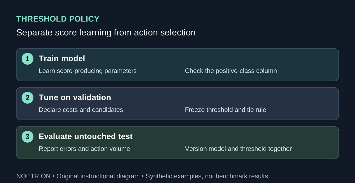
2. Derive the expected-cost rule under stated assumptions
Assume a binary outcome, a calibrated conditional probability p of the positive outcome, a false-positive cost C_FP, a false-negative cost C_FN, and zero cost for correct actions. Taking the positive action has expected cost (1-p) times C_FP. Taking the negative action has expected cost p times C_FN. Choose positive when the former is no greater than the latter.
Rearranging gives p greater than or equal to C_FP divided by (C_FP plus C_FN), provided the denominator is positive. For costs one and five, that boundary is one sixth. This is an algebraic consequence of the stated loss table. Different costs for correct actions, example-specific costs, capacity constraints, or uncalibrated scores require a different analysis.
import numpy as np

false_positive_cost, false_negative_cost = 1.0, 5.0
threshold = false_positive_cost / (false_positive_cost + false_negative_cost)
assert np.isclose(threshold, 1 / 6)
probabilities = np.array([0.10, 0.20, 0.80])
cost_if_positive = (1 - probabilities) * false_positive_cost
cost_if_negative = probabilities * false_negative_cost
decisions = probabilities >= threshold
assert np.array_equal(decisions, cost_if_positive <= cost_if_negative)
assert decisions.tolist() == [False, True, True]
print("Expected-cost boundary:", threshold)
The numbers in this fixture are probabilities supplied by us, not estimates whose calibration was measured. A real model's output requires calibration assessment on appropriate data before a probability-based interpretation is justified. Even well-calibrated development predictions may change meaning if the deployment population or outcome process changes.
3. Select an empirical policy on validation data
An empirical approach compares candidate thresholds using observed validation outcomes and a declared loss. It can be used for scores without treating them as calibrated probabilities. Its selected threshold is a fitted policy parameter: validation labels influenced it, so performance on those same labels is a development result rather than an independent final estimate.
import numpy as np
from sklearn.metrics import confusion_matrix

validation_y = np.array([0, 0, 1, 1, 1, 0])
validation_scores = np.array([0.10, 0.40, 0.30, 0.70, 0.90, 0.80])
candidates = np.array([0.20, 0.50, 0.85])

def loss(y, scores, threshold):
    predictions = (scores >= threshold).astype(int)
    tn, fp, fn, tp = confusion_matrix(y, predictions, labels=[0, 1]).ravel()
    return int(fp + 5 * fn), (int(tn), int(fp), int(fn), int(tp))

validation_losses = [loss(validation_y, validation_scores, t)[0]
                     for t in candidates]
assert validation_losses == [2, 6, 10]
selected = float(candidates[int(np.argmin(validation_losses))])
assert selected == 0.20
test_y = np.array([0, 1, 1, 0])
test_scores = np.array([0.15, 0.25, 0.75, 0.60])
test_loss, counts = loss(test_y, test_scores, selected)
assert test_loss == 1 and counts == (1, 1, 0, 2)
print("Frozen policy test loss:", test_loss, "counts:", counts)
The program chooses among three predeclared candidates using only validation values, then evaluates that fixed choice on a separate synthetic test fixture. It does not search again using the test outcomes. The six validation rows and four test rows are far too few to support a deployment claim; they make the data-flow boundary and arithmetic easy to audit.
The candidate set is also part of the procedure. Searching only three thresholds can miss a better validation operating point. Searching many candidates increases the amount of adaptation to validation noise. State the search resolution, tie-breaking rule, constraints, and objective when reporting the selected policy.
4. Compare decisions using the actual objective
| Policy element | Required definition | Common ambiguity |
|---|---|---|
| Positive class | Which outcome requires the positive action | Probability taken from the opposite class |
| Loss units | Consequence assigned to each error type | Treating illustrative costs as measured costs |
| Threshold operator | Whether equality selects positive | Different serving and evaluation behavior |
| Candidate search | Range, resolution, and tie-breaking | Unreported additional tuning |
| Evaluation boundary | Data untouched by fitting and selection | Reporting tuned validation loss as final performance |
The model evaluation guide documents metrics and scoring. Report the confusion counts alongside a scalar objective so readers can see what changed. Two policies can have the same total cost while distributing errors differently. If the operational question includes queue capacity or subgroup performance, cost alone may not describe suitability.
Use rates and counts together. A policy that is manageable in a low-volume validation sample may overload a queue at deployment volume. Precision also depends on the evaluated population's outcome prevalence. A threshold selected on a deliberately balanced sample may need a different operational analysis for a population with a much rarer positive outcome.
5. Keep model fitting, calibration, and tuning separate
The TunedThresholdClassifierCV reference describes cross-validated threshold selection. Its prefit option requires particular care: the data used to tune the threshold should be independent of the data used to fit the classifier. Selecting a threshold from overly optimistic in-sample scores can produce a policy that does not transfer to new observations.
When calibration, hyperparameter selection, and threshold tuning are all performed, diagram the complete procedure. Each adaptive step needs an appropriate boundary. Cross-validation can support development decisions, but simply calling several cross-validation utilities in succession does not automatically make every reported score independent of every decision.
Group structure and chronology remain relevant. Scores for multiple records from one entity can be highly related. A threshold for future activity should be assessed using information available before the outcomes being predicted. Store the selected threshold with the exact fitted score-producing model; a threshold learned for one model is not automatically appropriate for a refitted model with a different score distribution.
6. Monitor the frozen policy after deployment
Observe the rate of positive actions, queue load, outcome delay, and later error counts. A sudden shift in action rate can result from changed inputs, changed prevalence, a software problem, or a genuine process change. It is a diagnostic signal, not an automatic instruction to move the threshold until the dashboard looks familiar.
If a policy is updated, treat the update as a new selection procedure with its own validation and version. Preserve the former configuration so decisions can be traced to the policy in effect at the time. Record positive-class mapping, score source, threshold, comparison operator, costs, selection population, and package versions as one deployable contract.
Finally, acknowledge uncertain consequences. Operational costs may be estimated rather than known, and different stakeholders may value errors differently. Sensitivity analysis over plausible cost assumptions is more transparent than publishing one precise threshold as universally optimal. A defensible decision policy connects a stated objective to an auditable procedure and reports what the available evidence can actually support.
Sources and scope
The three official scikit-learn 1.8 references support threshold APIs and evaluation conventions. The expected-cost derivation and all synthetic arithmetic are original instructional examples. Neither program establishes production calibration, optimal operational costs, or a reliable final performance estimate from tiny samples.