A Precise Estimate of the Average Does Not Make the Next Observation Predictable
Separate uncertainty about a population mean from variation in a future observation. Follow a checked example and label interval targets before using a forecast.
A report estimates an average near 100 and gives a narrow interval around it. Someone uses that interval to plan the range of the next individual measurement. The number may have been calculated correctly while answering a different question.
A confidence interval for a population mean concerns uncertainty in an estimated average. A prediction interval for a new observation must also account for the variation of individual observations around that average. More data can improve the first without eliminating the second.
The NIST Dataplot references distinguish confidence limits for a mean from prediction limits for new observations. This guide uses an original normal-model example, checked on 26 October 2026, to show why choosing the target comes before choosing the formula.
Name the quantity that needs an interval
Are you estimating the average of a stable process, predicting one future item, or predicting the average of a future batch? Those are distinct targets even if they share a point estimate.
For example, a manager assessing long-run average processing time has a different question from a customer asking how long their next request might take. The same interval should not be copied between those decisions without checking what it describes.
Write the target in the chart label. “95% interval” is incomplete when the reader cannot tell whether it describes a parameter, a future observation or a collection of future outcomes.
Start with a deliberately simple model
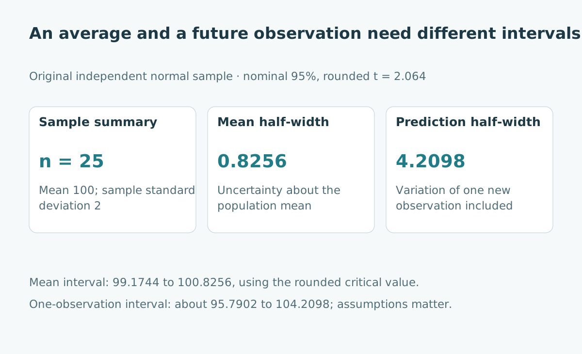
Assume 25 independent observations from an unchanged normal distribution. Their fictional sample mean is 100 units and sample standard deviation is 2 units. The population standard deviation is unknown and estimated from this sample.
Use a two-sided nominal 95% interval and a Student t critical value with 24 degrees of freedom. For transparent arithmetic, take the rounded value 2.064, consistent with the NIST t table.
| Original model input | Assumed value | Meaning |
|---|---|---|
| Sample size | 25 | Number of independent observations |
| Sample mean | 100 | Estimated population average |
| Sample standard deviation | 2 | Estimated individual variation |
| Rounded t critical value | 2.064 | Two-sided nominal 95%, 24 degrees of freedom |
These inputs are teaching summaries, not a measured production dataset. No trend, seasonality, covariate shift or measurement bias is included.
Calculate uncertainty about the mean
The standard error of the estimated mean is sample standard deviation divided by the square root of sample size. Here it is 2 divided by 5, or 0.4 units.
Multiply by 2.064 to obtain a half-width of 0.8256. The interval for the population mean is therefore 99.1744 to 100.8256 under the model and rounded critical value.
This is narrow because averaging independent observations reduces the variability of the mean estimator. It does not say that individual observations are squeezed into the same narrow range.
Add the variation of the next observation
For one new independent observation from the same normal population, the prediction half-width is the critical value multiplied by the sample standard deviation and the square root of one plus one divided by sample size.
The extra one represents the variation of the new observation. Using the original inputs gives approximately 4.2098 units, yielding a prediction interval of about 95.7902 to 104.2098.
| Target under the original model | Half-width | Interval around 100 |
|---|---|---|
| Population mean | 0.8256 | 99.1744 to 100.8256 |
| One new observation | About 4.2098 | About 95.7902 to 104.2098 |
Both calculations use the same sample. The wider prediction interval is not evidence that its analyst was less careful; it answers a more variable question.
Reproduce the arithmetic
This standard-library Python example uses the stated rounded critical value rather than silently selecting another distribution or confidence level.
from math import sqrt, isclose

n = 25
sample_mean = 100.0
sample_sd = 2.0
t_critical = 2.064  # Rounded two-sided 95% value, 24 degrees of freedom
mean_half = t_critical * sample_sd / sqrt(n)
prediction_half = t_critical * sample_sd * sqrt(1 + 1 / n)
assert isclose(mean_half, 0.8256)
assert round(prediction_half, 4) == 4.2098
assert prediction_half > mean_half
print("Mean interval:", sample_mean - mean_half, sample_mean + mean_half)
print("Next observation:", sample_mean - prediction_half,
      sample_mean + prediction_half)
Rounding the critical value affects the last digits. The point is the different variance terms, not an implied precision beyond the model or the available data.
Interpret coverage as a property of the procedure
Under the model, a 95% confidence procedure produces intervals containing the fixed population mean in 95% of repeated samples. It does not assign a 95% frequentist probability to the already-fixed mean after this particular interval has been calculated.
A prediction procedure instead targets coverage of a new random observation, accounting for uncertainty in the fitted quantities. Its nominal coverage also relies on the assumed population and sampling process remaining appropriate.
Neither statement guarantees a particular next measurement will fall inside its interval. An outside observation can occur under the model and may also be a reason to investigate whether the assumptions still fit.
Do not confuse prediction with process limits
An interval calculated from a sample is not automatically a specification limit, a contractual guarantee or an acceptable operating range. Those limits come from requirements and consequences, not merely from observed variability.
A process can be statistically stable while producing results outside a customer's tolerances. Conversely, one surprising observation does not by itself establish a permanent process change. Decide which question the analysis is intended to answer.
For a future batch average, the formula changes again because the target averages several new observations. State the future sample size; do not relabel the one-observation interval as a batch forecast.
Check whether independence and stability are plausible
Repeated readings from one device can be correlated. A daily demand series can have a trend. A mixture of distinct customer groups can be skewed or multimodal. Those situations can invalidate the simple normal-sample calculation.
More observations from a changing process do not automatically repair a misspecified model. Examine how the data were collected and whether the next case belongs to the same population.
The original example is useful precisely because its assumptions are visible. A real forecast may require an appropriate time-series or regression model, separate validation, and an interval method suited to the intended target.
Use the interval in the decision it actually supports
When planning around a future individual outcome, inspect an appropriate predictive distribution or interval and the cost of being wrong. When assessing an average effect, inspect the mean estimate and its uncertainty. Keep those results side by side when both matter.
For related tools, see regression error metrics and time-series validation gaps. A well-labeled interval becomes useful when its target matches the decision and its assumptions match the data.
Sources and limits
- NIST confidence limits for a mean.
- NIST prediction limits.
- NIST-hosted Student t critical-value table, Appendix A.
Sources checked 26 October 2026. The normal model, sample summaries and decision examples are original illustrations, not a validated forecast of a real process.