Inventory Buffers: Set the Reorder Point from Usable Lead Time
Build a practical reorder-point worksheet using usable delivery time, inventory position, and disruption tests, with exact examples and honest limits.
The ship has arrived, but the component is still unavailable. It may be waiting for clearance, inland transport, inspection, or release into production. A reorder rule based only on sailing time will miss those days, even when the shipment tracker looks reassuring.
The inventory decision is therefore about usable supply, not a headline transit estimate. Too little buffer can interrupt work; too much ties up cash and risks deterioration or obsolescence. A defensible reorder point begins by defining the clock correctly, then testing what happens when the delivery pattern changes.
Why the logistics evidence needs careful reading
The World Bank's Connecting to Compete 2025 publication record, dated April 22, 2026, introduces Logistics Performance Indicators 2.0 based on shipment-level operational data. The title year and publication year differ. Its methodology separates stages such as maritime transit, transshipment, and time at arrival facilities.
The current methodology page is useful because it makes the endpoints explicit. Port-to-port time is not the same as the full interval between placing an order and having acceptable stock ready for use. These indicators help diagnose logistics performance; they are not a promised lead time for your supplier or a ready-made safety-stock recommendation.
The World Bank's April 21, 2026 Trade Watch summary also describes supply-chain adaptation and relatively low shipping costs through February 2026 despite continuing pressures. That is historical context, not evidence that your route is cheap or reliable in October. Price and reliability must be measured separately.
Define the order-to-usable clock
For your operation, start the clock at the point relevant to the purchasing decision. If an order needs two days of internal approval before the supplier accepts it, include those days unless your reorder process genuinely eliminates them. End the clock when conforming stock can serve demand.
| Lead-time stage | Possible start and end | Evidence to collect |
|---|---|---|
| Internal approval | Reorder signal to released purchase order | System timestamps |
| Supplier preparation | Accepted order to dispatch | Supplier confirmation and actual dispatch |
| Main transport | Dispatch to destination arrival | Carrier events |
| Clearance and inland movement | Arrival to warehouse receipt | Clearance and receiving records |
| Acceptance | Warehouse receipt to usable release | Inspection outcome and release time |
Use one unit throughout: calendar days or working days. If demand occurs seven days a week but replenishment works only weekdays, converting between the two requires an actual calendar rather than a casual multiplier.
Rejected goods need special treatment. A delivery that fails inspection has not completed the usable-stock clock. If your records stop at the first physical arrival, they can make the supplier look more reliable than the production team experiences.
Use inventory position rather than the shelf count
A reorder rule usually needs inventory position: stock on hand plus valid outstanding replenishment, less unfilled demand already committed. The shelf count alone ignores orders on the way and obligations the stock must satisfy.
Suppose a fictional workshop has 420 units on hand, 180 units on an outstanding purchase order, and 70 units owed to customers. Inventory position is 530 units: 420 + 180 − 70. If the reorder point is 600, that position triggers action even though the warehouse physically contains 420 units.
The purchase order must be real and relevant. An overdue order with no credible delivery date should not be treated as equally useful to one confirmed for tomorrow. A basic inventory-position calculation does not solve time-phased availability: an order arriving after a stockout cannot prevent the stockout.
For that reason, keep both a position total and a dated view of expected arrivals. The position helps avoid duplicate ordering; the arrival schedule helps identify shortages before replenishment becomes usable.
Start with a transparent coverage calculation
Consider a fictional workshop consuming 40 units per calendar day. Its ordinary order-to-usable lead time is 12 days. Management provisionally selects an additional three days of demand coverage as a buffer. This is a chosen policy for the example, not a statistically estimated service level.
Expected lead-time demand is 40 × 12 = 480 units. The buffer is 40 × 3 = 120 units. The reorder point is therefore 600 units.
| Assumption or result | Fictional value | Interpretation |
|---|---|---|
| Daily demand | 40 units | Constant in the first calculation |
| Ordinary usable lead time | 12 calendar days | Whole process, not only transport |
| Chosen buffer | 3 days, or 120 units | Management assumption |
| Expected lead-time demand | 480 units | 40 × 12 |
| Reorder point | 600 units | 480 + 120 |
| Disrupted lead time | 18 calendar days | Separate stress assumption |
| Demand over disrupted lead time | 720 units | 40 × 18 |
| Gap relative to the original reorder point | 120 units | 720 − 600 |
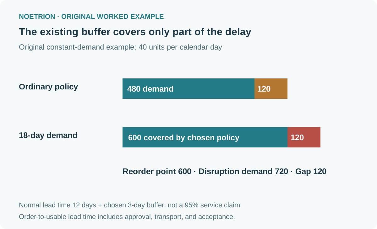
The extra six delivery days require 240 more units than the ordinary 480-unit demand. The existing 120-unit buffer covers only half of that extension. This is why “we already carry safety stock” is an incomplete answer to a changed lead-time pattern.
Separate the reorder point from the order quantity
The reorder point answers when to order. The order quantity answers how much to buy. Raising the reorder point does not automatically mean doubling every purchase order, and a large order quantity does not necessarily make a late reorder safe.
Suppose the workshop normally orders 400 units at a time. Under a simple steady-demand sawtooth model, that lot contributes average cycle stock of 200 units. With 120 units of buffer, approximate average on-hand inventory is 320 units. This approximation assumes regular replenishment, no persistent backlog, and the stated buffer behavior.
If the workshop increases the buffer to 240 units while keeping order quantity at 400, approximate average stock rises to 440. At a fictional landed cost of $25 per unit, the extra 120 units tie up $3,000. At an assumed annual carrying rate of 24%, the incremental annual carrying cost is $720.
The carrying rate is a modeling input, not a universal industry number. Depending on how your organization defines it, storage, financing, insurance, damage, and obsolescence may already be included. Avoid adding those costs twice. Minimum order quantities, warehouse capacity, and expiry dates can also make a simple coverage policy infeasible.
Do not label a chosen buffer as a 95% service level
Three days of buffer is not automatically “95% safe.” A service-level claim requires a defined metric, a relevant demand-and-lead-time model, and evidence that the assumptions are reasonable. Cycle service level—the chance of avoiding a stockout in a replenishment cycle—is different from the fraction of demand filled immediately.
Daily demand can rise precisely when deliveries become difficult. Treating demand and lead time as independent may understate the joint risk. Promotions, holidays, supplier shutdowns, and transport disruptions can also invalidate a single historical average.
For a small operation, begin with an honest empirical table. Record actual order-to-usable days and demand during each interval. Inspect the slow deliveries, not only the average. A sample of ten orders is useful operational evidence but a weak basis for confident claims about rare disruptions.
A stronger policy can use a distribution of demand during replenishment lead time rather than separately combining unrelated averages. The right method depends on the data, review frequency, shortage consequences, and item characteristics. The simple example here is a first diagnostic, not a replacement for a validated inventory model.
Compare a buffer with alternatives
Extra stock is one possible response. Others include reducing internal approval delays, improving visibility, qualifying another supplier, changing delivery frequency, or arranging an emergency shipment. Each has costs and constraints.
| Response | What it may improve | What to investigate first |
|---|---|---|
| More buffer stock | Coverage during delay | Cash, storage, ageing, and expiry |
| Faster approval | Internal part of lead time | Whether the delay is actually internal |
| Alternative supplier | Exposure to one source | Qualification, quality, and shared upstream dependencies |
| More frequent deliveries | Cycle stock and responsiveness | Freight cost and supplier capacity |
| Emergency transport | Recovery from a specific shortage | Availability, cost, and remaining clearance steps |
Two suppliers are not necessarily independent. They may rely on the same upstream component, port, or logistics provider. Likewise, paying for faster transport may leave the longest clearance or inspection delay unchanged. Map which stage an intervention can actually shorten.
You can compare the modeled $720 annual extra carrying cost with a proposed response, but do not assume the cheaper number is automatically better. The expected frequency and consequence of shortages matter. A safety-critical part and a replaceable decorative item should not receive an identical policy merely because their unit costs match.
Run a weekly exception review
A practical worksheet should show item, usable on-hand quantity, dated outstanding orders, committed demand, inventory position, reorder point, and next review date. Add an exception flag when an order becomes overdue or a supplier changes its confirmation.
At review, ask three questions: has demand changed, has the usable lead-time pattern changed, and is any supposedly available stock unusable? These questions catch problems a static formula can miss. Record who can authorize a temporary policy change and when that change expires.
For a reader exercise, use the fictional workshop. At demand of 50 units per day, the original 15-day combined coverage requires 750 units. If an 18-day disruption is also considered, demand would reach 900 units. Decide which assumption has changed and calculate the cash implication before proposing a larger buffer.
Then repeat with one real item using your own observations. Label missing data, separate normal and disrupted conditions, and keep the calculation visible. The goal is a policy you can revise when evidence changes, rather than a round number that survives only because nobody remembers how it was chosen.
The working capital worksheet shows how additional inventory can affect the cash gap.
Sources and verification notes
- World Bank, Connecting to Compete 2025 publication record, April 22, 2026: LPI 2.0's operational-data redesign.
- World Bank LPI methodology: different logistics-stage endpoints.
- World Bank Trade Watch, April 21, 2026: historical trade and shipping context, including the February measurement boundary.
Checked October 20, 2026. All workshop quantities, costs, and stress assumptions are synthetic and independently checked. No observed shortage probability, supplier promise, or guaranteed service level is claimed.