Correlation vs Causation: Reading Relationships and Simpson's Paradox
Explore correlation vs causation with charts, tables, and Simpson's paradox. Check confounding, study design, and the limits of conclusions from data.
Checked on October 2, 2026. Every exercise number was created for this article. None represents a course study or product-performance claim. Calculations are provided for reproduction.
A dashboard shows that participants spending more time in an application earn higher scores. The team concludes that increasing usage time will improve ability. That may be true, but the chart has not established it. More motivated participants may both use the application longer and study more diligently elsewhere.
Correlation describes a statistical relationship; causation concerns change resulting from an intervention. "Who uses the application longer?" differs from "What happens when comparable participants receive additional usage time?" That distinction guides data collection, comparison groups, and defensible conclusions.
Descriptive, predictive, and causal questions
All three tasks below are useful, but need different evidence. Descriptive reporting can identify a real pattern without claiming a cause. Prediction can work even when some variables are not causes. Evaluating an intervention needs additional justification that its comparison reflects the situation without that intervention.
| Question | Example | What to examine |
|---|---|---|
| Descriptive | Do usage time and scores move together? | Definitions, paired observations, plot shape |
| Predictive | Can first-week data predict completion? | Evaluation on new data and information leakage |
| Causal | Does a new exercise feature improve completion? | Feature assignment, comparison, timing, causal assumptions |
Do not turn successful prediction into an intervention claim. "Received a certificate" might predict completion extremely well, but issuing certificates early does not automatically teach the material. Variables available only after an outcome can also create data leakage.
What does Pearson correlation measure?
The SciPy pearsonr documentation describes Pearson's coefficient as a measure of linear relationship, ranging from −1 to 1. Positive values indicate a tendency to move together; negative values indicate opposing movement. The coefficient does not identify a causal mechanism.
Pearson summarizes a straight-line pattern. It can be zero for a U-shaped relationship. Consider synthetic pairs x = [-2, -1, 0, 1, 2] and y = [4, 1, 0, 1, 4]. Every y equals x squared, yet Pearson correlation is zero. It would be incorrect to conclude that no relationship exists.
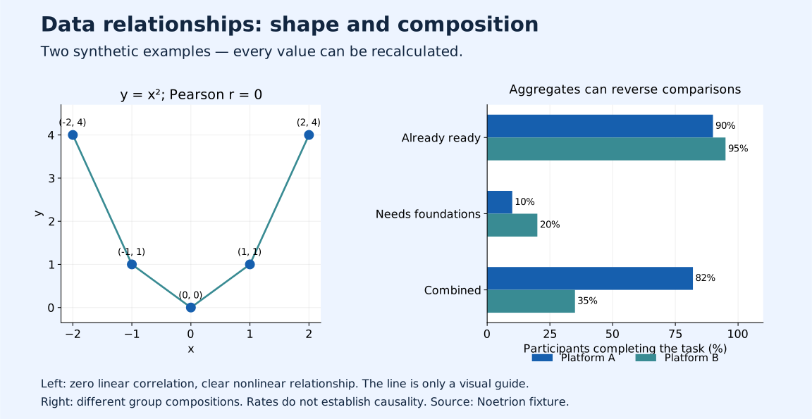
This example uses Python's statistics.correlation, available from Python 3.10. It computes a coefficient, not causality or a research design.
from statistics import correlation

x = [-2, -1, 0, 1, 2]
y = [4, 1, 0, 1, 4]
r = correlation(x, y)
assert abs(r) < 1e-12
print(round(r, 6))  # 0.0
Look at a scatterplot before reducing a relationship to one number. Examine units, outliers, observation range, and mixed groups. If x is constant, the coefficient is undefined; do not replace it with zero for a tidy table. Handle missing observations as pairs under an explicit policy rather than separately dropping x and y values and pairing different people.
Confounding: a shared cause
A confounder can affect both group assignment and the outcome. Prior ability may influence feature selection and final scores. If experienced participants dominate the new-feature group, its higher score cannot immediately be interpreted as a feature benefit.
Julia Rohrer's methodological article discusses causal models, shared causes, and observational-data limitations. Before inspecting every result, write down plausible mechanisms: who selects a group, when selection occurs, and what factors already existed? This helps avoid choosing explanations only after seeing attractive numbers.
Another teaching example: usage and scores might both rise during exam preparation. The study calendar becomes a candidate shared cause. Reverse direction is also possible: participants who understand the material may feel more comfortable using the application. A relationship observed in one period does not establish its causal direction.
Simpson's paradox with checkable numbers
Imagine course platforms A and B accept participants with different initial readiness. The outcome is completion of one task. This entire table is synthetic. Different group compositions were chosen deliberately to demonstrate an aggregate reversal.
| Readiness before the course | A: completed / participants | A rate | B: completed / participants | B rate |
|---|---|---|---|---|
| Already ready | 81 / 90 | 90% | 19 / 20 | 95% |
| Needs foundations | 1 / 10 | 10% | 16 / 80 | 20% |
| Combined | 82 / 100 | 82% | 35 / 100 | 35% |
B has a higher completion rate in both readiness groups. A nevertheless has the higher combined rate because 90% of its participants are already ready, compared with 20% for B. The aggregate arithmetic is correct. The mistake arises when that number answers a different question without accounting for composition.
A's rate is 0.90 × 0.90 + 0.10 × 0.10 = 0.82. B's is 0.20 × 0.95 + 0.80 × 0.20 = 0.35. Within each expression, participant proportions weight the group's completion rates.
Changes or reversals after splitting groups are discussed in Stanford Encyclopedia of Philosophy: Simpson's Paradox. The platform example is Noetrion's construction, not a copied empirical study. It illustrates weighting and says nothing about a real platform's effectiveness.
What if both compositions were the same?
For a descriptive standardization exercise, give both platforms 50% already-ready participants and 50% needing foundations. A's weighted rate becomes 50%; B's becomes 57.5%. The change follows from defining the same comparison population.
a_ready, a_foundations = 81 / 90, 1 / 10
b_ready, b_foundations = 19 / 20, 16 / 80

a_combined = (81 + 1) / (90 + 10)
b_combined = (19 + 16) / (20 + 80)
a_standardized = 0.5 * a_ready + 0.5 * a_foundations
b_standardized = 0.5 * b_ready + 0.5 * b_foundations

assert b_ready > a_ready and b_foundations > a_foundations
assert a_combined > b_combined
assert abs(a_standardized - 0.50) < 1e-12
assert abs(b_standardized - 0.575) < 1e-12
print(a_combined, b_combined, a_standardized, b_standardized)
Standardization still does not establish B's causal effect. We do not know whether readiness measurement is accurate, motivation differs, tasks have equal difficulty, or "completed" has a consistent definition. The 50/50 weights are exercise choices; real analysis needs a target population and justification for its weights.
Report percentages with participant counts. A denominator of ten has different uncertainty from thousands of participants. This small example demonstrates arithmetic structure only. It makes no significance, population-interval, or real-participant generalization claim.
Do not automatically control every column
Adding more regression variables does not guarantee less bias. The DAG primer by Rose and colleagues distinguishes confounders, mediators, and colliders. A variable on an intervention's mechanism path can be a mediator; adjusting for it changes the effect question. Controlling a collider can open a previously blocked association.
Group selection therefore needs justification from time ordering and domain knowledge. Our example measures readiness before the course. Grouping by "completed extra exercises" after platform assignment would have a different causal meaning. Do not select strata merely because they produce a preferred conclusion.
DAGitty offers resources for drawing causal assumptions and studying adjustment. A diagram makes assumptions visible, but does not prove its arrows correct. Record supporting knowledge and potentially unmeasured factors.
What evidence supports a causal claim?
Athey and Imbens' review of randomized experiments distinguishes assignment-based inference from sampling. In a feature experiment, random assignment prevents the assignment mechanism from systematically following initial ability, although chance imbalance remains possible. Random assignment concerns intervention comparisons; random sampling concerns whom a sample represents.
For a practical design, specify the primary outcome in advance, keep task versions comparable, and track attrition. Avoid stopping solely when an interim result becomes favorable. If experimentation is unavailable, observational analysis needs an explicit design and assumptions; adding "controlled for" to a report is insufficient.
A p-value does not determine causal truth. The American Statistical Association statement explains that a p-value is neither the probability a hypothesis is true nor a measure of effect size or importance. A statistically significant relationship can still have alternative explanations.
Write conclusions that match the evidence
| Overreaching claim | Appropriate wording for this example |
|---|---|
| A must be more effective because 82% completed | A has a higher aggregate completion rate in these synthetic data |
| B is proven to cause improvement | B is higher in both strata; the causal effect remains undetermined |
| Zero correlation means no relationship | This Pearson measure shows no linear relationship; the nonlinear pattern is visible |
| A small p-value proves causation | Interpret the test alongside design, assumptions, and effect size |
Before publishing a chart, state data origin, period, sample size, definitions, and missing-value policy. Use the Noetrion Data Explorer for initial inspection, then choose analysis appropriate to the design. These foundations do not replace a full causal evaluation for complex project decisions.
Sources and reproduction
Sources include SciPy/Python documentation, methodological and experiment literature, DAG resources, Stanford, and ASA, linked beside relevant explanations. The Python examples and table values were recalculated. Synthetic data does not represent a survey, experiment, or service-performance result.