NumPy Broadcasting: Make Shape Contracts Explicit
Verify broadcasting shapes, distinguish row and column offsets, and budget pairwise results with runnable NumPy examples.
Reviewed October 9, 2026. Examples target Python 3.12 and NumPy 2.3 and use synthetic arrays.
A calculation can produce a plausible array while applying every adjustment to the wrong observations. This is especially easy when a dataset happens to be square: a vector intended to describe rows also has the right length to describe columns. NumPy can check whether dimensions are compatible, but it cannot know what those dimensions mean in your application.
This tutorial treats shape as part of a data contract. The examples use small arrays whose expected values can be checked by hand. They are demonstrations of semantics, not benchmarks or evidence about a real population. By the end, you should be able to explain each axis before writing an expression, test its intended alignment, and estimate whether the result is affordable before allocating it.
1. Separate compatibility from meaning
NumPy compares dimensions from the right. A dimension can match an equal dimension or an axis of length one; missing leading dimensions behave as length one. These rules determine whether an operation is possible, rather than whether its interpretation is correct. A one-dimensional vector has no stored designation such as “row vector” or “column vector.” Its placement follows the expression and the shapes involved.
For a matrix whose axes mean observations and features, a vector of feature adjustments naturally aligns with the final axis. A vector of observation adjustments needs an explicit singleton feature axis. Writing that axis makes the repetition visible to readers. Naming variables after their role also helps: feature_offsets conveys more than b, although naming alone cannot prevent a wrong operation.
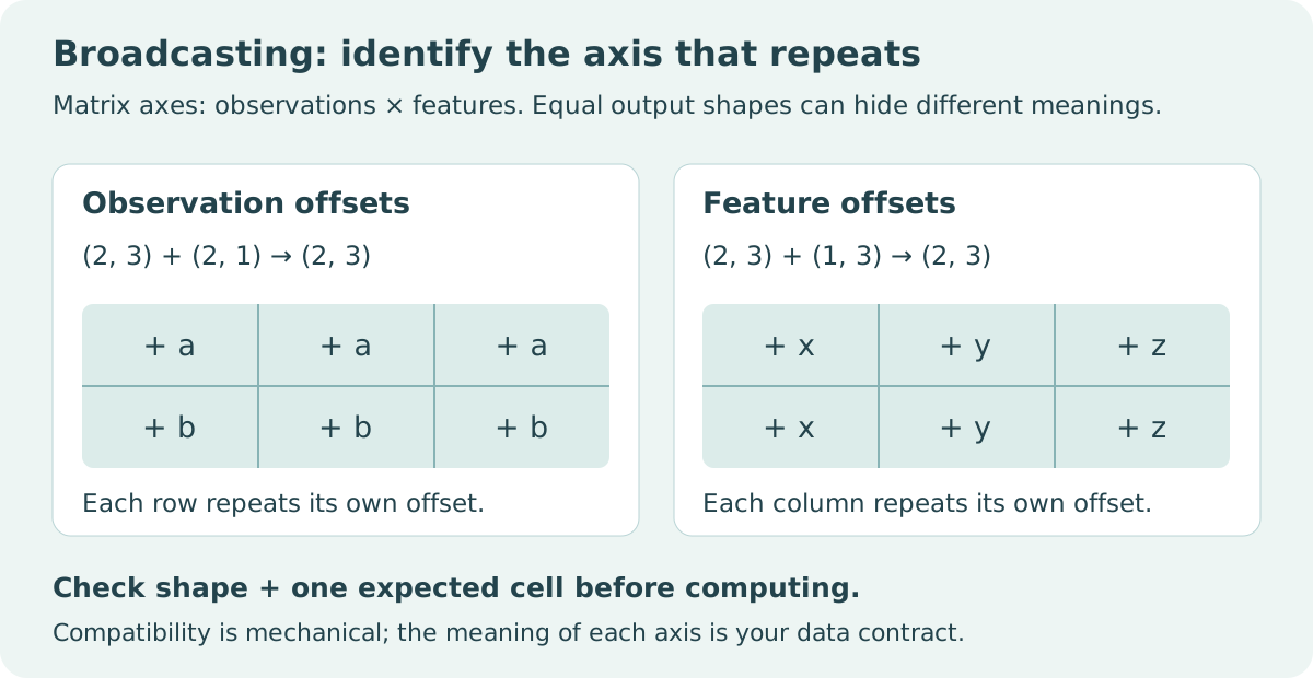
Treat the diagram as a review aid. Before evaluating an expression, write the intended output shape and one expected cell. If the first observation has values ten and twenty and its offset is one, the corrected row should be eleven and twenty-one. That concrete expectation catches a semantic error that a shape-only assertion would miss.
2. Test a square fixture that exposes ambiguity
The following program deliberately uses a two-by-two matrix. A non-square matrix often rejects an incorrectly shaped row vector immediately. A square fixture is more demanding because both interpretations fit, so the test must check values as well as dimensions.
import numpy as np

measurements = np.array([[10.0, 20.0], [30.0, 40.0]])
observation_offsets = np.array([1.0, 2.0])
feature_offsets = np.array([100.0, 200.0])

assert measurements.shape == (2, 2)
assert observation_offsets.shape == (2,)
assert feature_offsets.shape == (2,)
by_observation = measurements + observation_offsets[:, None]
by_feature = measurements + feature_offsets[None, :]
ambiguous = measurements + observation_offsets

np.testing.assert_array_equal(by_observation, [[11, 21], [32, 42]])
np.testing.assert_array_equal(by_feature, [[110, 220], [130, 240]])
np.testing.assert_array_equal(ambiguous, [[11, 22], [31, 42]])
assert not np.array_equal(ambiguous, by_observation)
assert np.broadcast_shapes((2, 2), (2, 1)) == (2, 2)
print(by_observation)
The last comparison is the essential test. It demonstrates a valid expression that violates our stated observation-level intention. An exception cannot protect this contract. The remedy is explicit orientation plus an expected-value fixture that distinguishes the two possible meanings.
| Adjustment meaning | Stored adjustment shape | Shape used in expression | Repetition |
|---|---|---|---|
| One value for each feature | (features,) |
(1, features) |
Across observations |
| One value for each observation | (observations,) |
(observations, 1) |
Across features |
| One value for the entire matrix | Scalar | () |
Across both axes |
| One value for every cell | Matrix | (observations, features) |
None required |
These are application conventions for a two-dimensional observation-by-feature matrix. A different axis ordering requires a different contract. Copying the syntax without checking the ordering merely moves the ambiguity elsewhere.
3. Validate inputs before adding axes
An explicit singleton dimension is useful only after the vector itself has been validated. Flattening arbitrary input to make an operation work can erase evidence that the caller supplied a matrix, an extra batch axis, or a malformed record. Prefer rejecting an unexpected number of dimensions to silently accepting every shape with the same number of elements.
A production helper could require a two-dimensional numeric matrix and a one-dimensional offset vector whose length equals the observation count. It should also decide whether missing values, infinities, and integer dtypes are allowed. Broadcasting does not make these decisions. An array can have the correct shape while containing values that violate the calculation's domain.
Keep axis order documented at boundaries such as file readers and model inputs. If one component provides feature-by-observation data while another expects observation-by-feature data, transposition should be a named transformation with its own check. Otherwise a coincidentally square input can conceal the mismatch for a long time.
4. Predict the result before allocating it
np.broadcast_shapes accepts shapes and returns the compatible result shape, raising ValueError for incompatible combinations. This makes it useful for a preflight check that does not need the full arrays. It does not validate axis meaning or guarantee that enough memory exists for the result.
For pairwise calculations, new singleton axes can create an output much larger than either input. Comparing every observation with every reference point produces an observation-by-reference grid. Keeping a feature axis during subtraction creates an additional dimension. Count the elements of that intermediate, multiply by the dtype's item size, and leave room for inputs, outputs, and other temporary arrays.
import numpy as np

observations = np.array([[0.0, 0.0], [3.0, 4.0], [1.0, 2.0]])
references = np.array([[0.0, 0.0], [3.0, 4.0]])
shape = np.broadcast_shapes(
    observations[:, None, :].shape, references[None, :, :].shape
)
assert shape == (3, 2, 2)
estimated_bytes = int(np.prod(shape)) * np.dtype(np.float64).itemsize
assert estimated_bytes == 96

full = ((observations[:, None, :] - references[None, :, :]) ** 2).sum(axis=2)
blocks = []
for start in range(0, len(observations), 2):
    block = observations[start:start + 2]
    squared = ((block[:, None, :] - references[None, :, :]) ** 2).sum(axis=2)
    blocks.append(squared)
chunked = np.concatenate(blocks, axis=0)
np.testing.assert_array_equal(chunked, full)
np.testing.assert_array_equal(full, [[0, 25], [25, 0], [5, 8]])

shared = np.broadcast_to(np.array([2.0, 3.0]), (3, 2))
assert shared.shape == (3, 2)
assert not shared.flags.writeable
print(full, estimated_bytes)
The ninety-six-byte figure describes only the synthetic subtraction-shaped array. It is not a peak-memory measurement. Squaring, reduction, retained blocks, and concatenation can require additional allocations. The chunked version establishes equality on the fixture; it does not establish a speed advantage on your hardware.
5. Distinguish repetition from materialization
np.broadcast_to provides a read-only view with the requested shape. Multiple logical positions can refer to the same underlying memory. This is why a broadcasted view is a poor place to express independent cell updates: the conceptual repetition does not create a separately owned value for every visible position.
An arithmetic result is a different question. Although broadcasting avoids a needlessly repeated input, a normal addition or subtraction still needs somewhere to place its result. A compact offset vector therefore does not imply a compact observation-by-reference output. Estimate the shape of every retained array, rather than considering only the smallest operand.
If downstream code genuinely needs a writable, independently stored expanded array, make that allocation deliberate and budget it. If downstream code only reads the repeated values, retaining the broadcasted view may be appropriate. Document that ownership decision so another function does not try to modify the view later.
6. Design chunking around the required answer
The example retains all block results because its purpose is to compare a complete grid. Many applications only need the nearest reference index or a reduction over references. In that case, storing the whole grid is unnecessary. A block can compute the needed reduction and discard its larger intermediate before the next block begins.
Define tie handling before implementing a nearest-reference calculation. Also consider whether feature scales make the distance meaningful; shape correctness does not establish the suitability of Euclidean distance. A unit mismatch can dominate a distance even when every axis is aligned perfectly.
Choose a block size using an explicit memory budget and a representative workload. Record the shapes and dtypes involved, then measure peak usage if the operational limit matters. The short fixture cannot provide a trustworthy default block size for large inputs, and vectorized syntax alone is not a performance guarantee.
7. Review the contract with adversarial fixtures
Use a square matrix, a single observation, a single feature, and an incompatible offset length when testing a helper. Distinct values in each row and column make orientation errors visible. An all-zero matrix or identical offsets often lets a faulty implementation pass because competing interpretations yield the same answer.
Assert both output shape and selected expected values. If missing or non-finite values are permitted, test their documented treatment separately. If they are rejected, test that rejection before arithmetic begins. A useful contract explains what the function accepts, how axes align, what it returns, and whether it allocates or shares memory.
The practical lesson is to make repetition intentional. NumPy supplies precise compatibility rules; your program supplies the meaning of each axis. Keeping those responsibilities explicit turns broadcasting from a compact trick into an auditable numerical operation.
Primary sources
- NumPy 2.3 broadcasting guide: dimensional compatibility and large-intermediate cautions.
- NumPy 2.3
broadcast_shapes: shape-only compatibility checks. - NumPy 2.3
broadcast_to: read-only broadcasted views and shared locations.