Averaging Two p95 Latencies Does Not Give You the Fleet's p95
Calculate a fleet p95 from original request data, see why weighted averages of percentiles fail, and choose histogram or raw-event evidence for aggregation.
Two servers report their p95 latency. A dashboard averages the two numbers and labels the result “service p95.” The display has combined summaries, but it has not reconstructed the request distribution from which the service percentile must be calculated.
Giving the busy server more weight does not generally repair the problem. Percentiles are not additive components. The missing information is where the individual observations sit when requests from all servers are ordered together.
The Prometheus histogram and summary guide explicitly distinguishes aggregatable distributions from precomputed summary quantiles. This article develops the arithmetic with original data so that the reason is visible, rather than asking readers to remember a monitoring rule without understanding it.
Name the population and the convention
A percentile needs a population. Are you measuring all completed requests, successful requests only, a particular route, or one customer's requests? It also needs a time window and a calculation convention.
For this tutorial, use the nearest-rank definition for p95: sort the observations and select rank equal to the ceiling of 0.95 times the number of observations, with ranks starting at one. Other conventions interpolate. NumPy's quantile reference documents several methods, which is why two tools can differ on a small sample without either calculation being a random error.
The example below does not rely on NumPy. Its integer rank calculation implements exactly the stated convention.
Pool the observations before selecting the rank
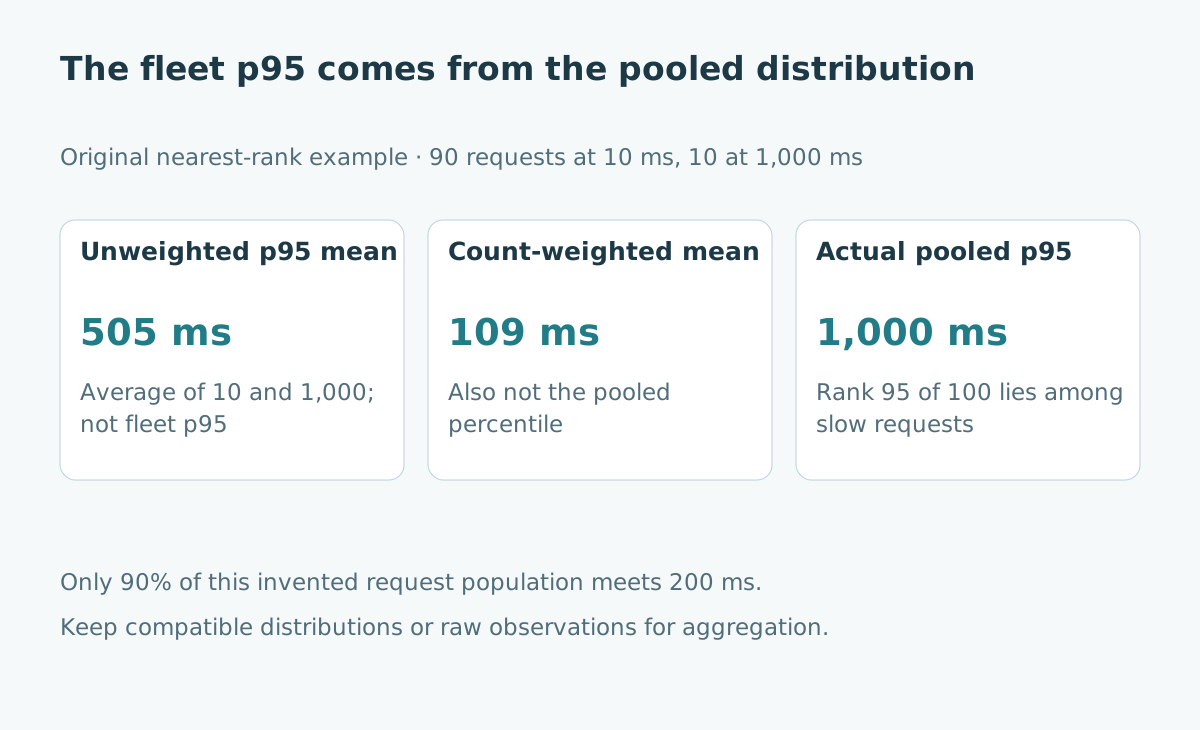
Server A handles 90 requests, all taking 10 milliseconds. Server B handles ten requests, all taking 1,000 milliseconds. The combined population contains 100 requests.
Ranks one through 90 are 10 milliseconds. Ranks 91 through 100 are 1,000 milliseconds. The nearest-rank p95 is observation 95, so it is 1,000 milliseconds.
| Fictional server | Request count | All observed latencies | Server p95 |
|---|---|---|---|
| A | 90 | 10 ms | 10 ms |
| B | 10 | 1,000 ms | 1,000 ms |
| Pooled fleet | 100 | 90 fast, 10 slow | 1,000 ms |
The pooled value describes a request drawn from the combined observed population. It is not an average experience of the two machines.
Try both tempting averages
The unweighted average of server percentiles is (10 + 1,000) / 2 = 505 milliseconds. That gives a server handling ten requests as much influence as the server handling 90. It does not select any rank in the pooled data.
The request-weighted average is (90 × 10 + 10 × 1,000) / 100 = 109 milliseconds. That is also not the pooled p95. In this specially constructed dataset, it happens to equal the pooled mean because every observation within each server is identical.
This coincidence should not become another shortcut. With more varied within-server distributions, a server p95 is not its mean, so even that equality disappears. Counts alone do not recover the information discarded by a percentile.
Reproduce the example in Python
The function below expects an already bounded, finite sample of non-negative integer or floating-point latencies. It rejects empty samples and invalid observations. It is an exact educational calculation over the supplied values, not a streaming monitoring implementation.
from math import isfinite


def p95_nearest_rank(sample):
    values = list(sample)
    if not values:
        raise ValueError("A percentile requires observations")
    if any(type(value) not in (int, float)
           or not isfinite(value) or value < 0 for value in values):
        raise ValueError("Latencies must be finite non-negative numbers")
    values.sort()
    rank = (95 * len(values) + 99) // 100
    return values[rank - 1]


a = [10] * 90
b = [1000] * 10
assert p95_nearest_rank(a) == 10
assert p95_nearest_rank(b) == 1000
assert p95_nearest_rank(a + b) == 1000
assert (p95_nearest_rank(a) + p95_nearest_rank(b)) / 2 == 505
assert (90 * p95_nearest_rank(a) + 10 * p95_nearest_rank(b)) / 100 == 109
assert sum(value <= 200 for value in a + b) / len(a + b) == 0.9
print("Fleet p95 is 1000 ms; only 90% of these requests meet 200 ms")
The last assertion answers a different but often useful question: what fraction of observed requests meets a chosen threshold? It is 90% here. Neither answer needs the misleading average of two percentiles.
Retain a distribution you can aggregate
If keeping every request is impractical, use a compatible distribution representation such as a histogram. Bucket counts preserve more information about the population than a single percentile does.
For example, cumulative counts at 50, 200 and 1,000 milliseconds would be 90, 90 and 100 for this toy sample. Those counts locate the 95th observation in the interval above 200 and at or below 1,000. They do not reveal its exact value without the raw data or additional assumptions.
Real histogram quantiles are estimates with behavior determined by the histogram type, bucket layout and query. Select a representation appropriate to the question and preserve the observation count alongside the result.
Align the measurement before combining it
Aggregation can be mathematically valid but operationally meaningless when the components describe different things. Check units, labels, time windows and inclusion rules before merging distributions.
| Check | Failure it prevents |
|---|---|
| Same unit | Mixing seconds with milliseconds |
| Same observation definition | Mixing queue wait with total request time |
| Same window | Combining one-minute and hourly views |
| Compatible distribution layout | Adding incompatible bucket populations |
| Consistent error handling | Silently excluding the slow failures |
Do not add cumulative bucket counts as though they were disjoint observations within a single histogram. Each observation contributes to all applicable cumulative upper bounds. Follow the monitoring system's documented aggregation semantics.
Keep timeouts and low counts visible
If a measurement records only completed requests, a timed-out request may disappear or be represented differently. A service can appear faster when its slowest requests stop reaching the timer's completion path.
Document how timeouts, cancellations and failures enter the measurement. Present their counts beside latency statistics. A percentile of successful completions cannot, on its own, represent the experience of every attempted request.
Likewise, a p95 from very few requests is sensitive to individual observations and the chosen convention. Always show the sample count and avoid interpreting small changes as established performance improvements without further evidence.
Choose an action tied to the request experience
For a latency objective, track the proportion meeting its threshold over the defined population. Use percentile views to investigate the tail, and segment by routes or workload classes when that reveals a meaningful bottleneck.
In the original example, investigating server B is sensible because it contains the observed slow requests. That does not prove the machine itself causes the delay. It may receive a different workload or wait on another system. Keep diagnosis separate from the summary statistic.
A defensible dashboard makes its population, units, window, count and method discoverable. The p95 is then a statement about ordered requests, rather than a convenient average of numbers that happen to share the same label.
Sources and further reading
- Prometheus: histograms and summaries, checked 25 October 2026.
- NumPy quantile methods, checked 25 October 2026.
- Related: profiling the actual bottleneck and data contracts.