PCA: Choose the Scale, Inspect Reconstruction, and Keep Prediction Claims Separate
Test PCA projection and inverse transformation, explain variance under a chosen scale, and fit dimensionality reduction inside training boundaries.
Reviewed October 9, 2026. Examples use Python 3.12, NumPy 2.3.5, and scikit-learn 1.8.0. The numerical arrays are synthetic.
Principal component analysis can turn several correlated measurements into fewer coordinates. A report may then call the first component the most important factor or describe a high explained-variance ratio as evidence of predictive success. Those conclusions exceed what the transformation actually measures. PCA describes variation in a selected numerical representation; it does not consult a target label when finding its directions.
The useful questions are more concrete: which units define the geometry, how much variation is retained, what reconstruction loses, and whether the transformed representation helps a separately evaluated downstream task. This guide answers the first three with transparent fixtures and explains how to investigate the fourth without allowing evaluation data to influence the transformation.
1. Start with the coordinate system
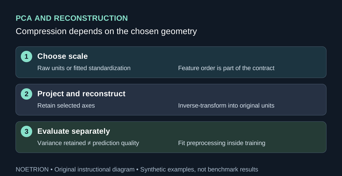
The PCA reference states that PCA centers input features but does not automatically scale each feature. Consequently, changing the units of one column can change the fitted directions. A measurement written in thousands and another written in fractions may contribute very different numerical variation.
Standardization is a modeling decision that gives nonconstant features a comparable fitted variance scale. It can be sensible when relative variation is the intended geometry, but it is not automatically the correct geometry for every scientific or operational question. A low-variance measurement may be precise and useful, or it may be mostly noise. Treating all standardized features equally does not resolve that distinction.
Write a feature dictionary before fitting: column name, unit, allowed range, missing-value policy, measurement process, and availability time. Exclude identifiers and arbitrary category codes unless there is a defensible numerical interpretation. A rotation of arbitrary codes produces arithmetic coordinates, but those coordinates need not encode a meaningful relationship between categories.
2. Verify projection and reconstruction on a line
import numpy as np
from sklearn.decomposition import PCA

X = np.array([[0., 0.], [1., 2.], [2., 4.], [3., 6.]])
model = PCA(n_components=1, svd_solver="full").fit(X)
coordinates = model.transform(X)
reconstructed = model.inverse_transform(coordinates)
assert coordinates.shape == (4, 1)
assert reconstructed.shape == X.shape
assert np.allclose(reconstructed, X)
assert np.isclose(model.explained_variance_ratio_[0], 1.0)
assert np.allclose(model.components_ @ model.components_.T, [[1.]])
print("Reconstruction squared error:", np.sum((X - reconstructed) ** 2))
All four points lie on one affine line, so one centered direction can represent them completely apart from floating-point error. The fixture demonstrates the mechanics of transform and inverse_transform. It does not show that real observations occupy a line or that measurement noise can always be discarded safely.
The component direction is a unit-length axis in feature space, while transformed values are coordinates along that axis after centering. The signs of an axis and its coordinates can reverse together without changing the reconstructed points. Do not interpret a sign reversal across equivalent fits as proof that the underlying phenomenon reversed. Compare the represented subspace and reconstruction when signs are arbitrary.
3. Make the scale change visible
The next array deliberately gives the second feature much larger numerical variation. It contains balanced, independent variation along both axes. Raw PCA prioritizes the second axis; after standardization, both contribute equally to total variance in this exact fixture. Equal variance also means the orientation within the tied subspace is not uniquely informative.
import numpy as np
from sklearn.decomposition import PCA
from sklearn.preprocessing import StandardScaler

X = np.array([[-1., -100.], [-1., 100.],
              [1., -100.], [1., 100.]])
raw = PCA(n_components=1, svd_solver="full").fit(X)
assert raw.explained_variance_ratio_[0] > 0.999
assert np.isclose(abs(raw.components_[0, 1]), 1.0)
scaler = StandardScaler().fit(X)
scaled = scaler.transform(X)
model = PCA(n_components=1, svd_solver="full").fit(scaled)
assert np.isclose(model.explained_variance_ratio_[0], 0.5)
scaled_reconstruction = model.inverse_transform(model.transform(scaled))
original_units = scaler.inverse_transform(scaled_reconstruction)
assert original_units.shape == X.shape
assert np.isclose(np.mean((scaled - scaled_reconstruction) ** 2), 0.5)
assert np.allclose(scaler.mean_, [0., 0.])
print("Raw and standardized retained ratios:",
      raw.explained_variance_ratio_[0], model.explained_variance_ratio_[0])
A retained ratio near one in the raw representation therefore does not imply that essentially every meaningful distinction was preserved. It means most of the numerical variance under that representation was retained. The first feature may matter to a target even when its contribution to raw total variance is small.
The StandardScaler documentation describes the fitted centering and scaling state. Preserve that state with the PCA model. Inverse transformation from component coordinates must first return to the scaled feature space and then undo scaling if values are to be interpreted in original units.
4. Define reconstruction error before reporting it
Reconstruction compares the original representation with the approximation recovered from retained coordinates. Specify whether the report uses a sum or mean, whether it averages over samples, features, or both, and whether values are measured before or after standardization. Without those definitions, two numbers called reconstruction error can describe different quantities.
| Quantity | Useful interpretation | Limitation |
|---|---|---|
| Retained variance ratio | Fraction of fitted variance represented by selected axes | Depends on feature scale and fitting data |
| Scaled reconstruction error | Lost variation in standardized coordinates | Does not preserve original physical units |
| Per-feature original-unit error | Approximation quality for each measurement | Different units should not be added casually |
| Downstream validation score | Performance of a specific predictive workflow | Requires labels and an appropriate split |
For measurements with different physical units, report per-feature errors or justify any common weighting used to aggregate them. Adding squared temperatures to squared lengths is arithmetic but not automatically an interpretable scientific loss. A product can choose a weighted approximation objective, provided the weights and their operational meaning are explicit.
Also inspect individual rows. A small average error can coexist with large errors for unusual but important observations. Reconstruction diagnostics should include the population to which they apply and the treatment of missing or outlying measurements. An unusual row can reflect a valid rare case, a changed process, or a data problem; the error alone cannot decide among them.
5. Keep unsupervised fitting inside the boundary
When PCA is part of a predictor, fit preprocessing and PCA on training data only. A pipeline allows each cross-validation fold to learn its own means, scales, and axes. Fitting the transformation once on the complete dataset before cross-validation uses evaluation-set structure and changes the claimed experiment, even though no labels were supplied to PCA.
Choose the component count using development data and the objective that matters. A variance-retention target is a compression criterion; a predictive score is a task criterion. They need not select the same number of components. Compare a baseline without PCA where feasible, rather than assuming fewer dimensions must improve prediction.
The decomposition guide places PCA among related transformations. A dense, centered numerical fixture should not be treated as a template for every sparse text matrix or nonlinear relationship. Select an algorithm and solver compatible with the actual representation and resource constraints, then document that selection.
6. Interpret axes cautiously and preserve the artifact
A component is a direction assembled from feature loadings, not a discovered causal variable. Naming it requires additional domain evidence. An axis with large loadings on several related measurements may summarize a recognizable pattern, but alternative measurements, scaling, or sampling can change that pattern. Avoid presenting a convenient label as something the algorithm proved.
Nearly tied components can rotate within a similar subspace when the dataset changes slightly. If stability matters, compare fitted subspaces or downstream behavior across appropriate resamples. Inspect whether an axis is dominated by a measurement artifact, such as a batch effect or a change in units, before describing it as a substantive phenomenon.
Store feature order, preprocessing state, fitted PCA parameters, selected component count, solver, version, and evaluation design together. Apply future observations with transform rather than fitting a fresh PCA independently and sending incompatible coordinates into the old classifier. The practical result is a reproducible compression contract whose information loss and predictive claims can each be assessed on their own evidence.
Sources and scope
The three official scikit-learn 1.8 references support the documented transformation APIs. The arrays, scale comparison, reconstruction calculations, and reporting guidance are original instructional material. Their exact numerical assertions demonstrate mechanics on synthetic points, not the quality of an unseen dataset or a causal interpretation of components.