Predictive Maintenance: When an Alert Is Worth an Inspection
Evaluate predictive maintenance with false-alarm counts, intervention lead time, and an original expected-cost example before authorizing deployment.
A vibration model can flag a machine before a fault becomes obvious. Whether that alert improves operations depends on what happens next: someone must interpret it, obtain access, arrange a suitable intervention, and finish while useful time remains. A high test score cannot answer all those questions.
NIST lists Comprehensive evaluations of condition monitoring-based technologies in industrial maintenance: A systematic review as published July 9, 2025. Its authors selected 42 eligible studies from 465 relevant papers covering 2001–2023 and found substantial differences in evaluation and economic reporting. NIST publication record. This is foundational evidence with a defined literature window, checked on October 14, 2026; it is not a breaking announcement or a census of every subsequent deployment.
Define the decision before the model score
Start with a maintenance decision that exists in the plant. “Inspect this bearing during the next available window” is evaluable. “Use AI to optimize reliability” is too broad to connect an output to a cost or an operational result.
Specify the equipment, fault type, prediction horizon, and existing maintenance policy. A detector of present anomalies is different from a prediction of failure within thirty days. Neither automatically provides remaining useful life. A maintenance team also needs an action threshold and an owner for each alert.
| Evaluation layer | Question | Evidence to collect |
|---|---|---|
| Signal | Does the sensor measure the intended phenomenon? | Calibration, placement, missing-data records |
| Prediction | Does an alert identify the defined target? | Held-out event counts and timing |
| Workflow | Can the team act in time? | Inspection queue, parts, access, completion times |
| Outcome | Does the policy improve the chosen result? | Costs and equipment outcomes against a baseline |
This original framework separates capabilities that are often compressed into one accuracy number. A good sensor can feed a poor model; a good model can feed an overloaded inspection team.
False alarms depend on the base rate
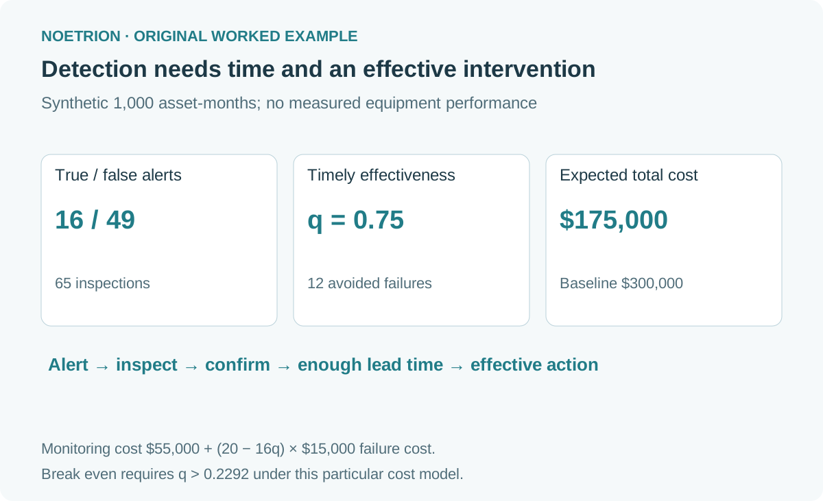
Consider a fictional fleet producing 1,000 nonoverlapping asset-month decisions. Assume 20 intervals would contain the defined failure under the comparison policy. The model has 80% sensitivity and 95% specificity on representative held-out data. These values are teaching inputs, not reported equipment performance.
| Actual condition under the comparison policy | Alert | No alert | Total |
|---|---|---|---|
| Failure within the defined horizon | 16 | 4 | 20 |
| No failure within that horizon | 49 | 931 | 980 |
| Total | 65 | 935 | 1,000 |
Sensitivity captures 16 of 20 failure intervals. The 5% false-positive rate produces 49 alerts among 980 nonfailure intervals. Only 16 ÷ 65 = 24.6% of alerts identify a future failure in this simplified untreated comparison.
That proportion does not mean the detector is useless. It means a workflow sized for sixteen inspections would be undersized: it receives sixty-five alerts. Teams should measure actionable cases and investigation effort together.
In real logs, repeated alerts for one episode must be grouped using a predefined rule. Counting the same developing fault every hour can inflate detection totals without creating additional opportunities to act. Likewise, an intervention changes the outcome, so a later absence of failure cannot automatically be relabeled as proof that the earlier alert was false.
Translate the alerts into expected cost
Assume each inspection costs $200, a planned intervention after a true alert costs $2,000, and an unplanned failure costs $15,000. The failure cost includes the selected downtime and repair categories; the planned-intervention cost includes its corresponding disruption. Add $10,000 for the monitoring service over these 1,000 decisions.
Let q be the assumed fraction of true alerts followed by a timely, effective intervention that avoids the modeled unplanned failure. Start with q = 0.75. This assumption must be measured in a pilot; the model's sensitivity does not establish it.
The comparison policy costs 20 × $15,000 = $300,000 for the modeled failures. With monitoring, expected cost is:
65 × $200 + 16 × $2,000 + (20 − 16q) × $15,000 + $10,000.
At q = 0.75, twelve of the sixteen alerted cases receive an effective, timely intervention in expectation. Eight failures remain: four missed cases and four unsuccessful or late actions. Total expected cost is $175,000, producing a hypothetical reduction of $125,000.
This is an intentionally narrow incremental comparison. Costs common to both policies cancel. It charges the planned intervention for every true alert, including unsuccessful ones, and assumes false alarms stop after inspection. If false alarms trigger replacement, or the baseline already includes preventive work, change the model before using it.
Test the intervention assumption
| Assumed timely, effective fraction q | Expected monitoring-policy cost | Difference from $300,000 baseline |
|---|---|---|
| 1.00 | $115,000 | $185,000 lower |
| 0.75 | $175,000 | $125,000 lower |
| 0.50 | $235,000 | $65,000 lower |
| 0.25 | $295,000 | $5,000 lower |
| 0.20 | $307,000 | $7,000 higher |
Break-even occurs when q exceeds $55,000 ÷ (16 × $15,000) = 0.2292 under these assumptions. The $55,000 comprises inspections, planned interventions, and monitoring. A threshold that catches more events can still lose value if it overwhelms the queue and reduces timely action.
Cost sensitivity matters too. With q held at 0.75 and failure cost reduced to $5,000, the baseline is $100,000 and the monitoring policy is $95,000. The apparent advantage shrinks to $5,000. The model did not change; the operational economics did.
These scenarios illustrate why uncertainty belongs beside the headline estimate. The NIST review discusses incomplete cost categories and limited uncertainty treatment, rather than establishing a universal savings rate. Full review, economic-analysis discussion
Lead time is part of usable detection
A warning two hours before failure may be technically correct and operationally unusable when parts require three days. Measure the interval from the first actionable alert to the event, then compare it with the entire response time: triage, confirmation, parts, access, and intervention.
For an original example, suppose the response needs four hours of triage, eight hours to confirm the fault, twenty-four hours for parts, and twelve hours to reach an access window. A serial workflow requires forty-eight hours before intervention can begin. An alert with twenty-four hours of warning cannot support that sequence. Parallel tasks may shorten it, but only if the actual process supports overlap.
Record a lead-time distribution rather than just an average. A seven-day average can conceal a subset of alerts arriving too late. Treat sensor outages, delayed transmission, and inspection backlogs as workflow failures that may reduce q.
Use decision gates before expanding deployment
An original pilot checklist turns these calculations into observable decisions:
- Define fault episodes, the prediction horizon, and the comparison maintenance policy before scoring.
- Split evaluation data by time and equipment where appropriate; prevent information from a later failure leaking into earlier predictions.
- Run a shadow period that records alerts and queue demand alongside the existing authorized policy.
- Reconcile labels with inspections and service records, including uncertain cases and interventions that alter outcomes.
- Introduce a bounded, authorized intervention pilot with predefined cost and response-time measures.
- Expand only when the observed evidence meets those decision criteria; retain an owner for ongoing review.
Report sensitivity, false alarms per decision or operating hour, actionable-alert yield, and lead time together. When fault counts are small, show the counts and uncertainty instead of presenting a percentage with misleading precision. Preserve equipment and operating-condition breakdowns so a fleet average cannot hide a weak subgroup.
Make a bounded deployment decision
The hypothetical cost result supports investigating an inspection policy, not claiming that failures will be prevented. A review should identify which assumptions are measured, estimated, or still unknown. It should also name who can pause the workflow if sensor quality, alert volume, or intervention capacity changes.
Prediction earns operational value through an executable action and a measured outcome. A deployment decision becomes reviewable when the team can trace an alert to inspection effort, available lead time, intervention results, and a defined cost comparison.
Sources and scope
- NIST publication page, July 9, 2025: authors Mehdi Dadfarnia, Michael Sharp, and Jeffrey Herrmann; study window 2001–2023.
- Author manuscript hosted by NIST: systematic-review methods and economic-analysis discussion; journal DOI.
All fleet counts, performance values, response times, and dollar amounts are original hypothetical inputs. Expected counts can be fractional in other scenarios. The calculation does not model correlated failures, uncertain labels, discounting, safety consequences, or the full lifecycle cost of a monitoring installation.