How Return Correlation Changes the Diversification of a Two-Asset Portfolio
Calculate a two-asset portfolio's volatility, inspect overlapping exposures, and test correlation assumptions without turning historical relationships into guarantees.
Educational analysis, not a personal investment or payment recommendation. Check the dated sources and the rules that apply in your jurisdiction.
Two funds can have different names and still depend on many of the same companies, currencies or economic conditions. Adding the second name may change the statement more than it changes the underlying exposure. Diversification therefore needs a question about relationships: what happens to the holdings together?
Investor.gov's allocation guide recommends looking inside funds, including whether their main holdings overlap. It also distinguishes spreading investments across asset categories from spreading them within a category. The count of products alone cannot establish either kind of diversification.
This evergreen guide uses an original two-asset calculation and a small scenario worksheet. All return, volatility and correlation inputs are assumed. They are not current market estimates, product rankings or a recommended allocation.
Start with comparable returns and weights
Define each holding's return over the same period and in the same reporting currency, with a consistent treatment of distributions. Otherwise, a correlation calculation can compare unlike quantities. An equity price-only series and a bond total-return series do not use the same return definition.
For a single holding period, the portfolio return is the sum of each asset's return multiplied by its beginning weight. Suppose half the portfolio starts in asset A and half in B. Its return is 0.5 × return_A + 0.5 × return_B, ignoring fees and trading during the period.
Those starting weights are assumptions for the calculation. A portfolio that is not rebalanced can have different weights in later periods. A strategy that rebalances needs its own timing, transaction-cost and tax assumptions.
Understand the relationship measured by correlation
Correlation summarizes a linear relationship between return variations. Positive values indicate that the returns tend to move together relative to their averages; negative values indicate an opposing tendency. Zero correlation does not establish statistical independence or eliminate the possibility of simultaneous losses.
Volatility measures the dispersion of returns. Covariance combines the relationship with the scale of each asset's variation. Two assets with the same correlation can contribute differently to portfolio variability if their individual volatilities differ.
The MIT portfolio-choice recitation presents portfolio variance as a weighted combination of variances and covariances. The example here applies that relationship using different, invented inputs rather than reproducing its worked exercises.
Calculate the two-asset variance before taking a square root
For weights w_A and w_B, individual standard deviations s_A and s_B, and correlation rho, the variance is:
w_A² × s_A² + w_B² × s_B² + 2 × w_A × w_B × rho × s_A × s_B.
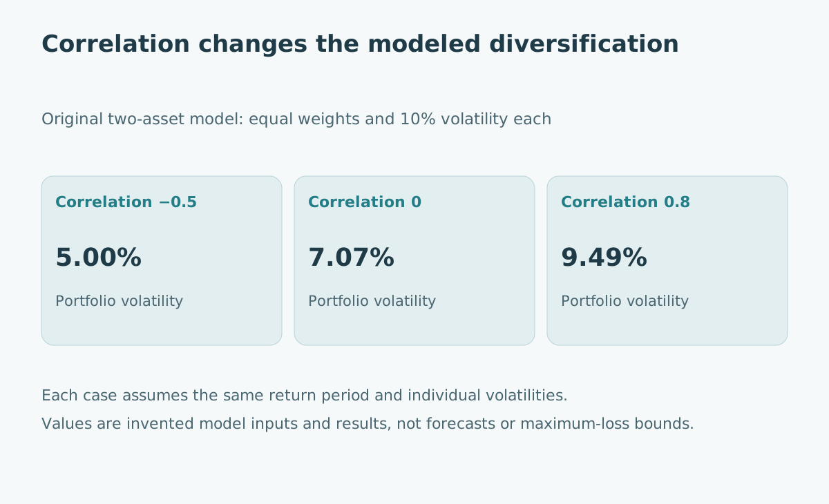
Use decimal returns consistently. A standard deviation of 10% enters as 0.10, not 10. With both weights equal to 0.5 and both standard deviations equal to 0.10, variance becomes 0.005 × (1 + rho). The portfolio standard deviation is the square root of that quantity.
| Assumed correlation | Portfolio variance | Portfolio standard deviation |
|---|---|---|
| −0.5 | 0.0025 | 5.00% |
| 0.0 | 0.0050 | About 7.07% |
| 0.8 | 0.0090 | About 9.49% |
| 1.0 | 0.0100 | 10.00% |
The same two holdings appear in every row. Changing only their assumed relationship changes the modeled diversification benefit. Averaging the two individual standard deviations would miss that relationship entirely.
Keep expected return separate from this risk calculation
Add another original assumption: A has a 6% expected return and B has an 8% expected return over the same holding period. The equal-weight portfolio's expected return is 7% in every row of the table. Correlation enters the variance calculation, not that weighted mean.
This does not mean a real portfolio can obtain an attractive relationship for free. Product prices, expected returns, fees and available exposures need their own analysis. The exercise simply holds them fixed to isolate one variable.
Nor is a standard deviation of 7.07% a promise that losses cannot exceed 7.07%. Variability, downside loss, liquidity and the ability to meet a spending commitment are different questions. A distributional model and additional assumptions would be needed for probability statements; none is supplied here.
Treat historical correlation as an estimate with a period
Record the data source, observation frequency, sample dates and return definition whenever presenting an estimated correlation. A longer sample contains more observations but can also combine different environments. A short sample may react quickly while remaining unstable.
A historical BIS analysis by Lombardi and Sushko discusses the shift toward positive US equity–government-bond correlation beginning in 2021 and its connection with the inflation environment. This is evidence that the relationship can change, not a current estimate for the reader's portfolio or proof that all bonds always move with equities.
For a sensitivity review, change the assumed correlation while keeping the other inputs visible, as the table does. Call the results conditional scenarios. Selecting the most reassuring historical window would not establish that its relationship will persist.
Add a loss scenario that does not require a correlation estimate
Suppose an invented adverse period produces returns of −20% for A and −15% for B. The equal-weight portfolio loses 17.5%. In a different hypothetical period, A loses 20% while B gains 5%; the portfolio loses 7.5%.
These are two arithmetic scenarios, not observations used to estimate correlation or probabilities assigned to future events. They help a reviewer ask whether the resulting loss is compatible with a stated commitment. A single paired outcome cannot identify a stable correlation.
Investor.gov's diversification explanation makes the broader limitation explicit: diversification cannot guarantee protection from a falling market. A scenario worksheet should retain that possibility rather than turn a lower modeled variance into a safety label.
Inspect the exposures behind the product labels
Create an original inventory with one row per meaningful exposure: underlying issuers, sectors, currency, interest-rate sensitivity, leverage and liquidity terms where relevant. For pooled products, inspect the available holdings and mandate rather than classifying them only by marketing name.
Ask whether a new holding adds an exposure you intended or duplicates one already present. Also identify information gaps. A stale holdings report is not a current, complete position file; an unexplained fund label does not fill that gap.
Costs belong beside the exposure review. Two products providing similar exposure can still have different fees or trading frictions. The investment-fee guide addresses that separate calculation, while index concentration and market breadth explains why a broad-looking index may have concentrated return drivers.
Write a decision record with conditional claims
An inspectable conclusion might state that a proposed combination has lower modeled variance under specified inputs, contains identified overlapping holdings and remains vulnerable to the listed adverse scenarios. Keep estimated relationships separate from assumed alternatives.
Update the review when exposures, liquidity needs or the decision horizon change. The purpose is to understand the portfolio's dependencies well enough to make a defensible choice, not to find a correlation number that makes an existing preference appear optimal.
Sources and scope
- Investor.gov, Asset Allocation and Diversification, official SEC investor education; scope and overlapping-fund guidance checked 31 October 2026.
- MIT OpenCourseWare, Portfolio Choice recitation, teaching material; portfolio mean, covariance and variance relationships reviewed.
- Lombardi and Sushko, The correlation of equity and bond returns, historical BIS analysis; discussion of the post-2021 relationship reviewed, not used as a current forecast.
- Investor.gov, Diversify Your Investments, official educational explanation of diversification's limits; checked 31 October 2026.
The numerical model, inventory and adverse outcomes are original illustrations. They do not select investments, quantify a particular portfolio's actual risk or provide personalized allocation advice.