Slowing a Pump by 20% Does Not Automatically Cut the Plant's Energy Bill by 48.8%
Use pump affinity laws without confusing shaft power with plant energy savings. Compare system curves, static head, operating time and delivered duty.
A variable-speed-drive proposal contains an attractive calculation: reduce pump speed to 80% and power falls to 0.8 cubed, or 51.2% of its original level. The arithmetic is correct. Whether it predicts the installation's energy use depends on what the pump must actually accomplish.
A plant buys a service: moving a required quantity of fluid while meeting pressure and process conditions. It pays for electricity over time. Neither requirement is fully described by a single speed ratio.
The US Department of Energy's adjustable-speed pumping tip sheet presents the affinity relationships and explicitly warns against directly using them to predict new operating points in systems with static head. This older engineering guidance was checked on October 26, 2026; it is not presented as a new rule or a current equipment recommendation.
State what must remain the same
Before comparing operating modes, define the useful output. Is the job maintaining circulation, filling a tank, transferring a fixed batch or meeting a changing process demand?
These are different comparisons. Ten hours at lower flow may deliver less fluid. A longer operating period may recover the original volume while changing the energy total. A lower discharge pressure may be unacceptable even when the motor uses less power.
An original assessment note should specify the volume, allowable pressure range, timing and fluid conditions. Without that service definition, a reduction in power could reflect reduced useful work rather than improved efficiency of the required task.
Use the affinity laws at corresponding points
For the same centrifugal pump with unchanged impeller geometry, ideal similarity gives flow proportional to rotational speed, head proportional to speed squared and shaft power proportional to speed cubed when efficiency is unchanged.
Let the speed ratio be 0.8. Then the corresponding-point ratios are:
| Quantity | Ideal ratio calculation | New value as a share of original |
|---|---|---|
| Rotational speed | 0.8 | 80% |
| Flow | 0.8 | 80% |
| Head | 0.8² | 64% |
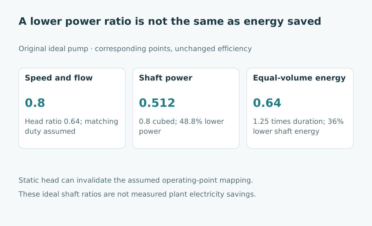
| Shaft power | 0.8³ | 51.2% |
These relationships map corresponding points on pump performance curves. They do not establish that the connected system will operate at the mapped point. That requires another piece of information: the system's head requirement at each flow.
Find the intersection with the system curve
The operating point is where the pump's available head meets the system's required head at the same flow. Changing speed shifts the pump curve. Opening a valve or changing a tank level can change the system condition.
For an original simplified comparison, normalize initial flow to one and initial head to 100 units. A friction-only system has head requirement 100 times normalized flow squared. At flow 0.8, that requirement is 64 units, matching the ideal corresponding head in this particular construction.
Now consider a different system with 40 units of static requirement plus 60 times flow squared. At the original flow of one, it also requires 100 units. At flow 0.8, however, it requires 40 + 60 × 0.64 = 78.4 units.
Notice what static head changes
The mapped pump point offers 64 units at flow 0.8, while the second system requires 78.4 units there. Those cannot describe the same operating point. A full reduced-speed pump curve is needed to locate the new intersection; the example does not calculate it.
| Original simplified system | Head at normalized flow 1 | Required head at flow 0.8 |
|---|---|---|
| Friction only: 100 × flow² | 100 | 64 |
| Static plus friction: 40 + 60 × flow² | 100 | 78.4 |
The DOE pumping sourcebook emphasizes evaluating the complete pumping system, including changing requirements and component interactions. The two original curves above show why a similar baseline operating point does not imply similar behavior after a speed change.
Static requirement does not disappear just because speed falls. The appropriate question is whether the proposed operating envelope still delivers the necessary duty.
Convert power into energy over the required time
Return to the ideal friction-only case. Suppose original shaft power is 100 kW for ten hours, delivering a fixed fluid volume. Original shaft energy is 1,000 kWh.
At 80% flow, delivering the same volume takes ten divided by 0.8, or 12.5 hours. With ideal shaft power of 51.2 kW, shaft energy becomes 51.2 × 12.5 = 640 kWh. That is a 36% reduction in this ideal equal-volume comparison, rather than 48.8%.
If the service instead requires lower flow for the same ten hours, shaft energy would be 512 kWh, but the delivered volume would also be lower. Neither scenario is a measured electricity saving. Motor and drive efficiency, operating limits and the actual duty profile remain outside these ratios.
Compare the actual control alternatives
A useful baseline is the installation's actual control method. It might throttle flow, use a bypass, cycle on and off, operate parallel pumps or already vary speed.
The comparison should ask what each option does while meeting the same accepted service. An assumed full-speed baseline can exaggerate an opportunity if the plant does not operate that way. A short favorable test can also miss conditions that dominate annual consumption.
Record the operating schedule and the reason for each mode. Distinguish changes attributable to production demand from changes attributable to control strategy. A lower monthly electricity total after a quieter production month does not isolate a drive's effect.
Build a measurement sheet around the duty
An original worksheet can contain time interval, required flow, measured flow, relevant head measurements, speed, electrical input power and accepted process output. Add the configuration of valves and parallel equipment.
Use the same measurement boundary for the baseline and proposed operation. Shaft-power relationships cannot simply be relabeled as meter readings. Establish how measurement accuracy and missing intervals affect the conclusion.
Before a trial, define acceptance conditions and the responsible engineering review. Flow, equipment limits, suction conditions and process constraints matter alongside electricity use. This article provides a reasoning framework, not instructions to change an industrial system without installation-specific assessment.
Present savings as an evidence-backed comparison
A defensible proposal identifies the useful duty, measured baseline, modeled alternative, assumptions and conditions that still need testing. It separates expected savings from observed savings.
The cube law is valuable as an engineering relationship and an initial screening tool. Its value increases when the report explains where it applies and where the actual system requires a fuller model.
For another example of local speed versus complete output, see robot cycle time and production throughput. For the boundary between model behavior and deployed evidence, see digital-twin validation.
Sources and evidence limits
- US DOE: Adjustable Speed Pumping Applications, Tip Sheet 11, January 2007. Supports the affinity relationships and static-head caution.
- US DOE and Hydraulic Institute: Improving Pumping System Performance, second edition, May 2006. Provides the systems-assessment foundation.
Both sources were checked October 26, 2026. All normalized curves and energy figures are original teaching examples, not vendor guarantees, equipment qualification or measured annual savings.